[1] "sf" "tbl_df" "tbl" "data.frame"Points live in a space: the CRS
Basic element of vector data: points. They can represent:
- self-standing features (e.g. bus stops);
- or be combined into lines and polygons.
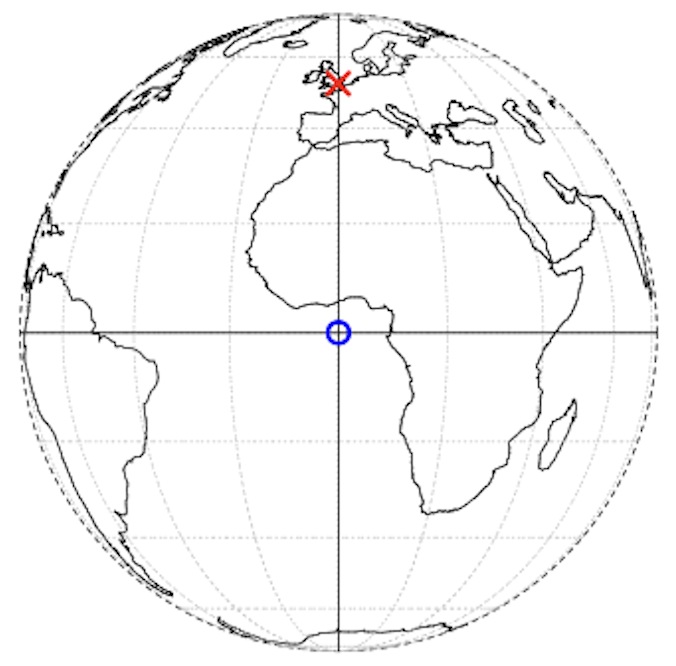
A point is identified by coordinates within a coordinate reference system (CRS).
Coordinates only make sense once a reference system is specified.
- For example, in a CRS London \(\rightarrow\) c(-0.1, 51.5)
- its location is 0.1° West and 51.5° North (w.r.t. Greenwich Prime Meridian and Equator).
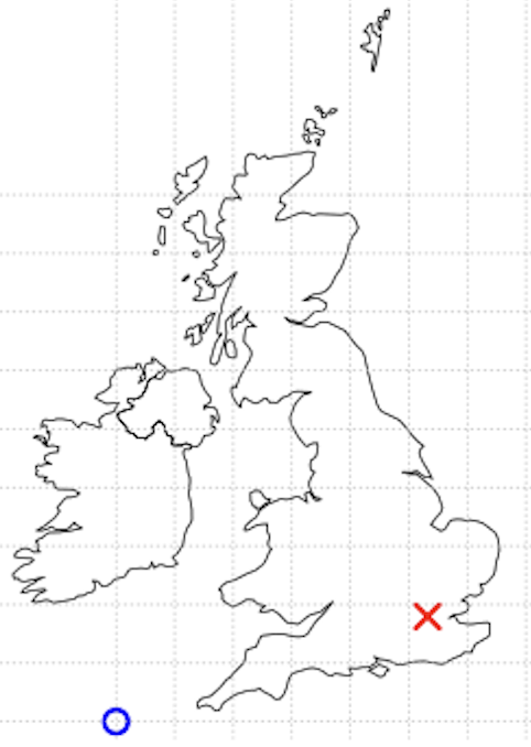
- In another CRS (British National Grid) London \(\rightarrow\) c(530000, 180000)
- 530 km East and 180 km North w.r.t another origin.
- For example, in a CRS London \(\rightarrow\) c(-0.1, 51.5)
Basic maps with sf
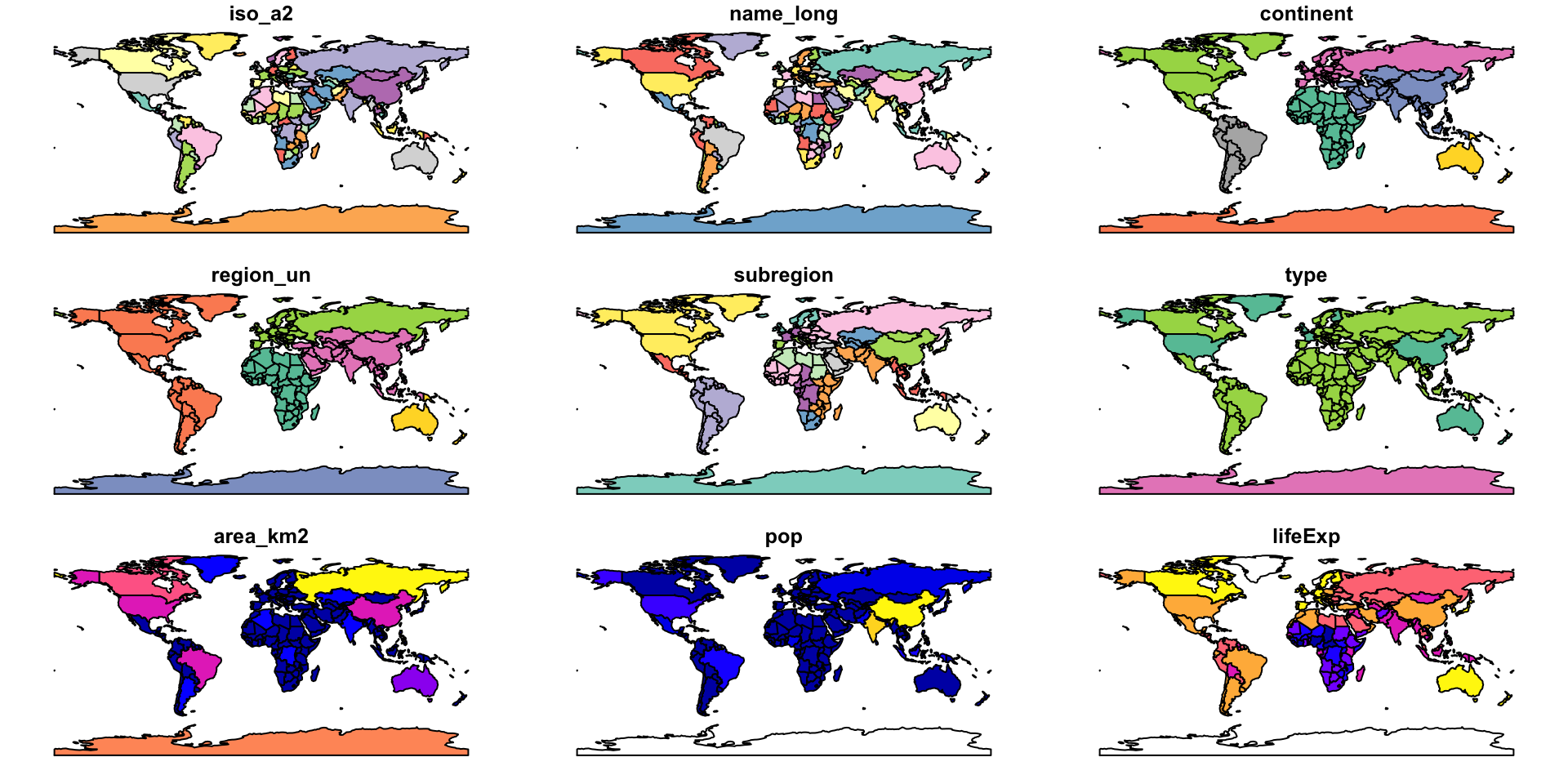
The default plotting methods make spatial exploration immediate.
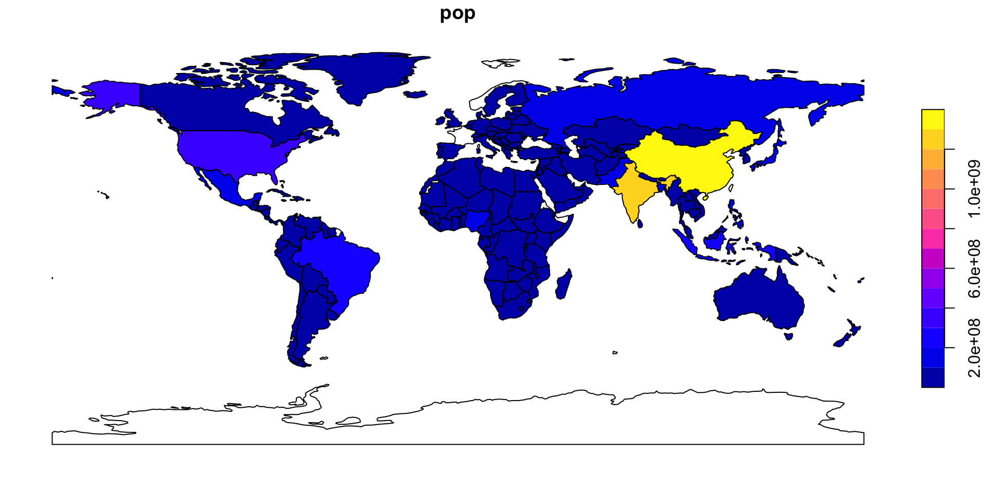
using ggplot you can create much nicer maps!
But let’s take a step back…
Geometry types
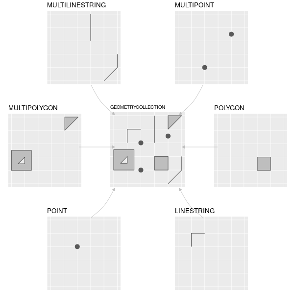
Geometries are the basic building blocks of simple features (hence the name sf).
Vector geometries are built from a few basic elements:
POINTLINESTRINGPOLYGON
And their multi-part versions:
MULTIPOINTMULTILINESTRINGMULTIPOLYGON
Creating geometries
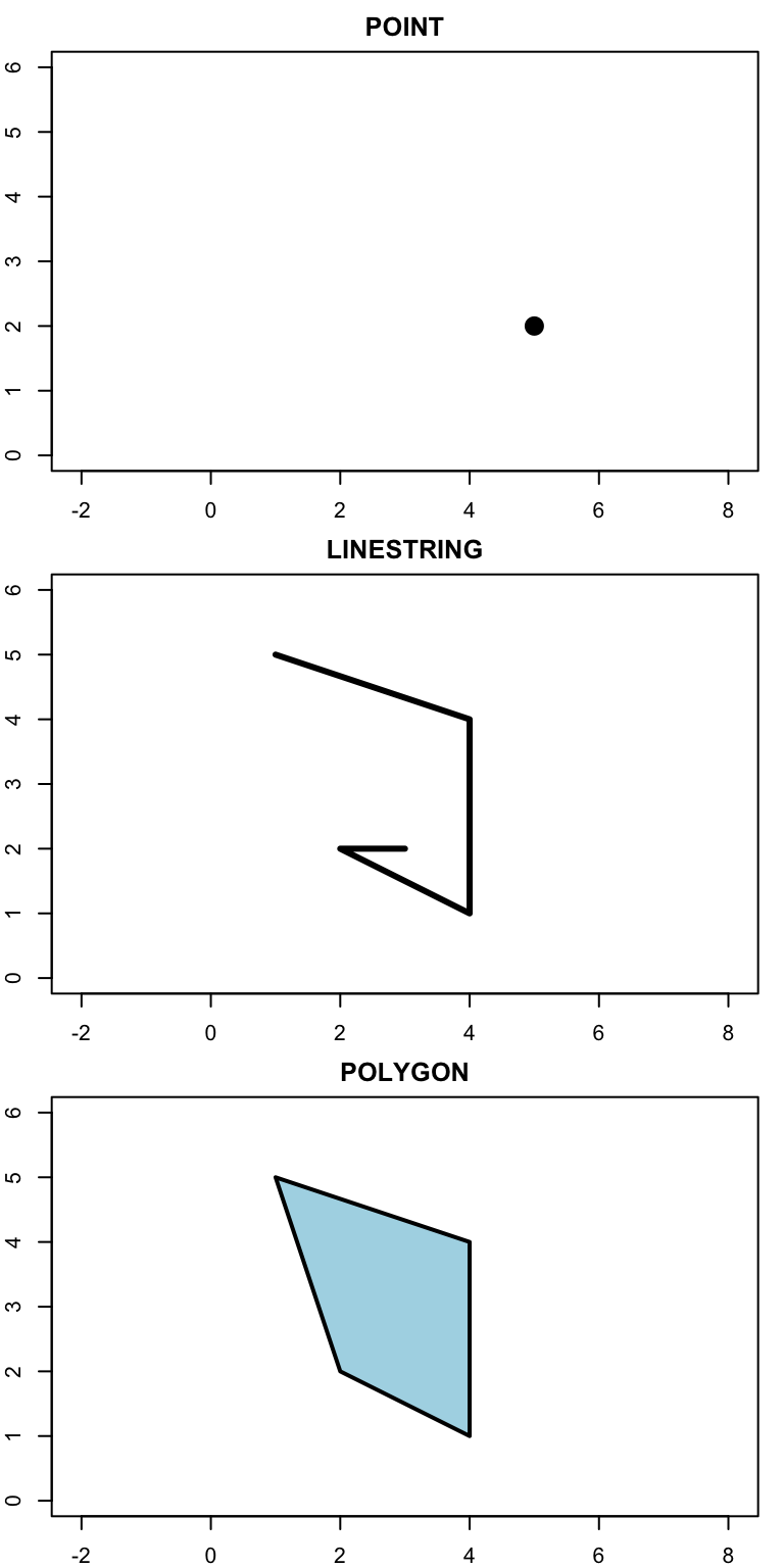
- A point is given by coordinate in two dimensions
- A linestring is a sequence of points with a straight line connecting them
- A polygon is a sequence of points that form a closed, non-intersecting ring.
Creating geometries II
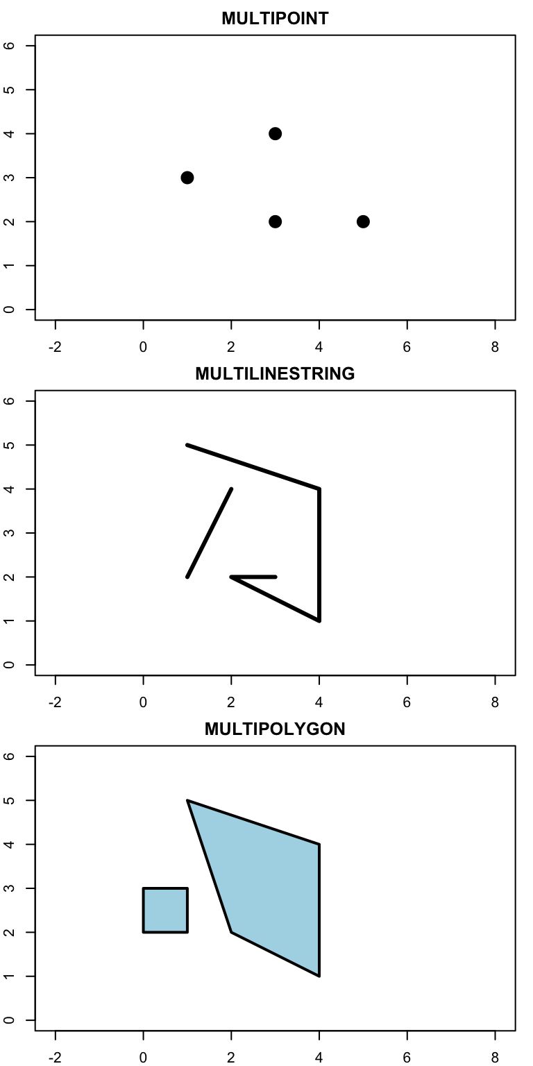
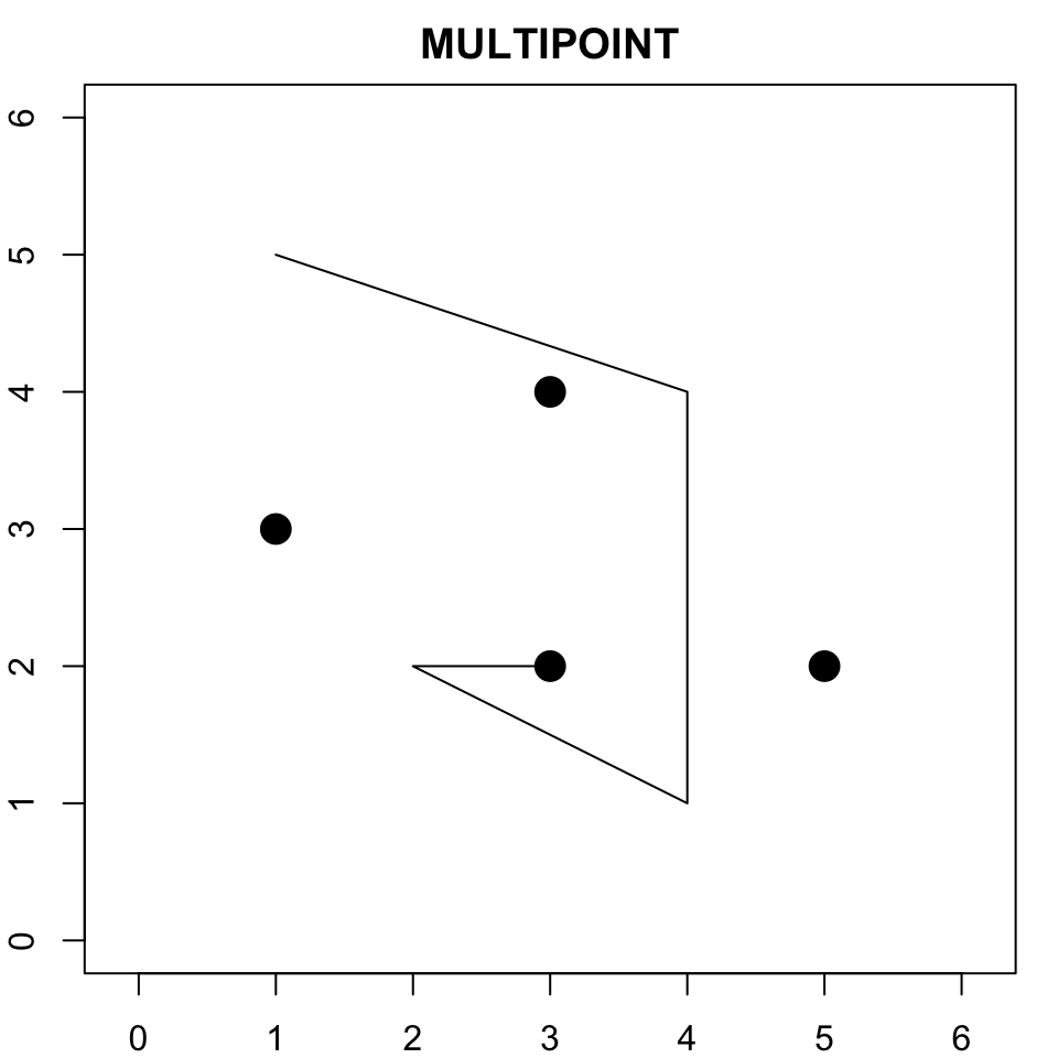
- Simple feature standard also allows multiple geometries of a single type to exist within a single feature within “multi” version of each geometry type.
- Use rbind for points, a list of rbinds of lines, and a list of a list of rbinds for polygons.
multipoint <- st_multipoint(
  rbind(
    c(5, 2),
    c(1, 3),
    c(3, 4),
    c(3, 2)
  )
)

multilinestring <- st_multilinestring(
  list(
    rbind(
      c(1, 5),
      c(4, 4),
      c(4, 1),
      c(2, 2),
      c(3, 2)
    ),
    rbind(
      c(1, 2),
      c(2, 4)
    )
  )
)

multipolygon <- st_multipolygon(
  list(
    list(
      rbind(
        c(1, 5),
        c(2, 2),
        c(4, 1),
        c(4, 4),
        c(1, 5)
      )
    ),
    list(
      rbind(
        c(0, 2),
        c(1, 2),
        c(1, 3),
        c(0, 3),
        c(0, 2)
      )
    )
  )
)
Creating geometries III
From sfc to spatial objects (sf, or simple features)
An sf object combines:
- a table of attributes;
- a geometry column
sfc.
#| class: small-code
rome_point <- st_point(c(12.4964, 41.9028))       # sfg object

rome_geom <- st_sfc(
  rome_point,
  crs = "EPSG:4326"
)                                                 # sfc object

rome_attrib <- data.frame(
  name = "Rome",
  temperature = 30,
  date = as.Date("2023-06-21")
)                                                 # data.frame object

rome_sf <- st_sf(
  rome_attrib,
  geometry = rome_geom
)

rome_sf
Geographic coordinates: WGS84
Which CRS should we use?
There is no universally “correct” CRS: the choice depends on the application. Anyway, most of the time the answer is WGS84 (EPSG:4326). Used by GPS systems; online maps; global spatial datasets.
Geographic CRS are not planar coordinates
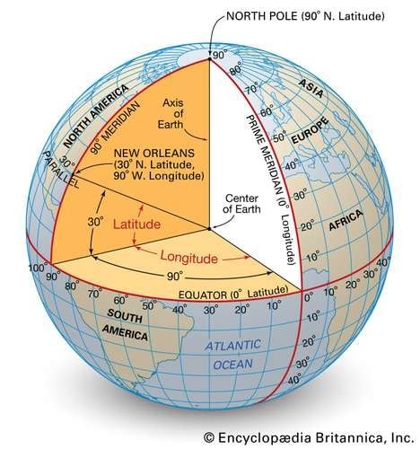
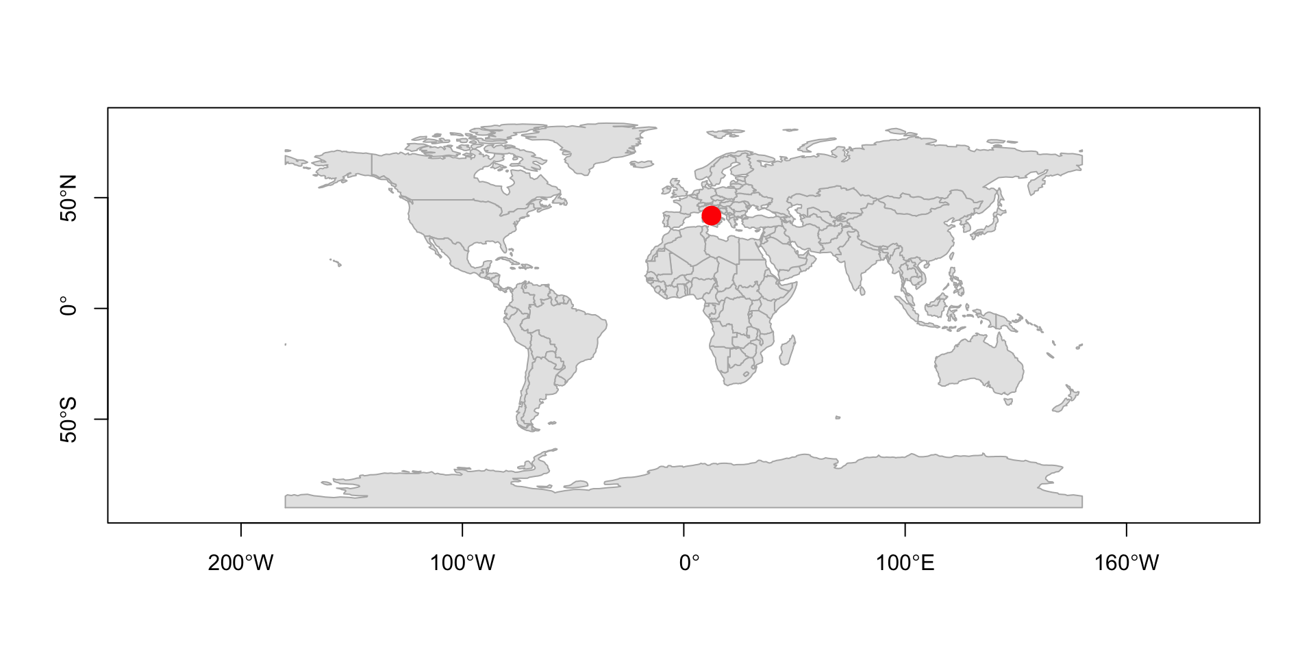
Longitude and latitude are angles, not distances.
A simple plot treats coordinates as if they were Cartesian
Bear in mind that degrees of longitude do not correspond to constant distances on Earth –> meridians converge toward the poles.
- 1° longitude at the Equator ≈ 111 km
- 1° longitude close to London ≈ 69 km
- 1° longitude close to North Pole ≈ 0 km
- Degrees of latitude are instead approximately constant in distance (1° ≈ 111 km)Every projection distorts the Earth
“All happy families are alike; each unhappy family is unhappy in its own way.”
- Lev Tolstoj, Anna Karenina.
“Each projection is in distorted in its own way”.
- Me, in this lecture
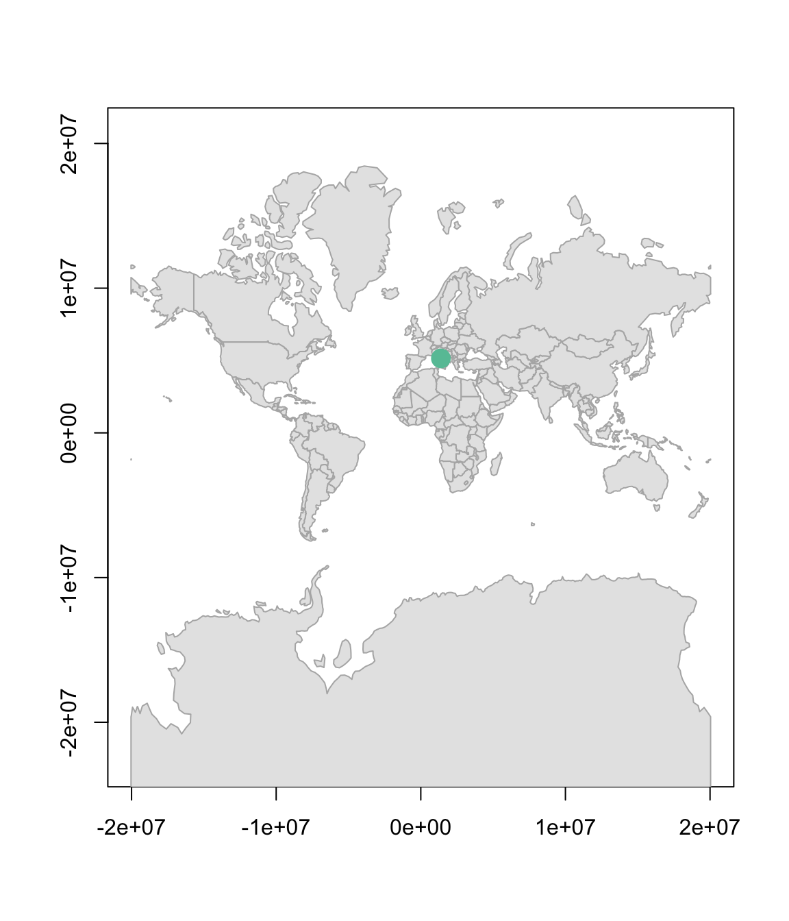
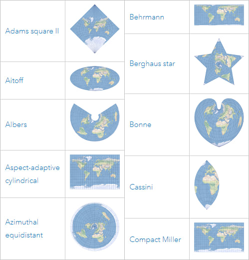
Why is Antarctica so big?
No flat map can preserve all geographic properties simultaneously.
Different projections preserve different properties: shape; area; distance; direction.
Geometry operations in sf
Modern versions of sf can use two different geometry engines.
This can affect the outcome of spatial operations.
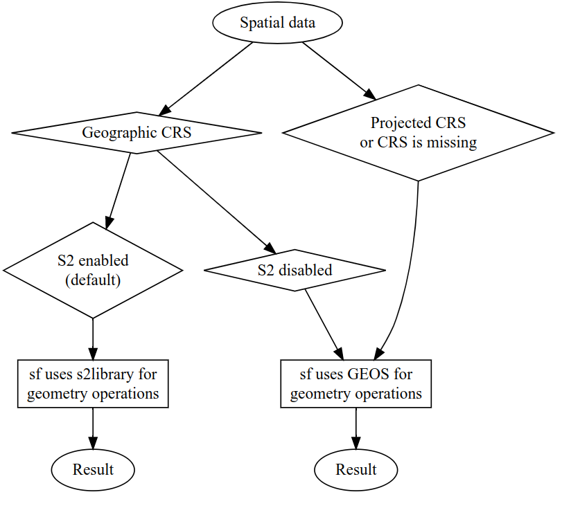
- Geographic CRS (
EPSG:4326) can use the spherical geometry engineS2; - Projected CRS typically use planar geometry (
GEOS); - Spatial operations therefore depend on both:
- the CRS;
- the geometry engine.
Why projections still matter
With S2 enabled (default), many operations on geographic CRS work well directly on the sphere.
With S2 disabled, some geometry operations (often involving distances, areas, buffers) may become problematic because longitude and latitude are treated as planar coordinates.
Generally, projected CRS are often more convenient for:
- local analysis (for small enough regions, the Earth is approximately flat)
- planar geometry operations;
- distances and buffers;
- spatial algorithms based on Euclidean geometry.
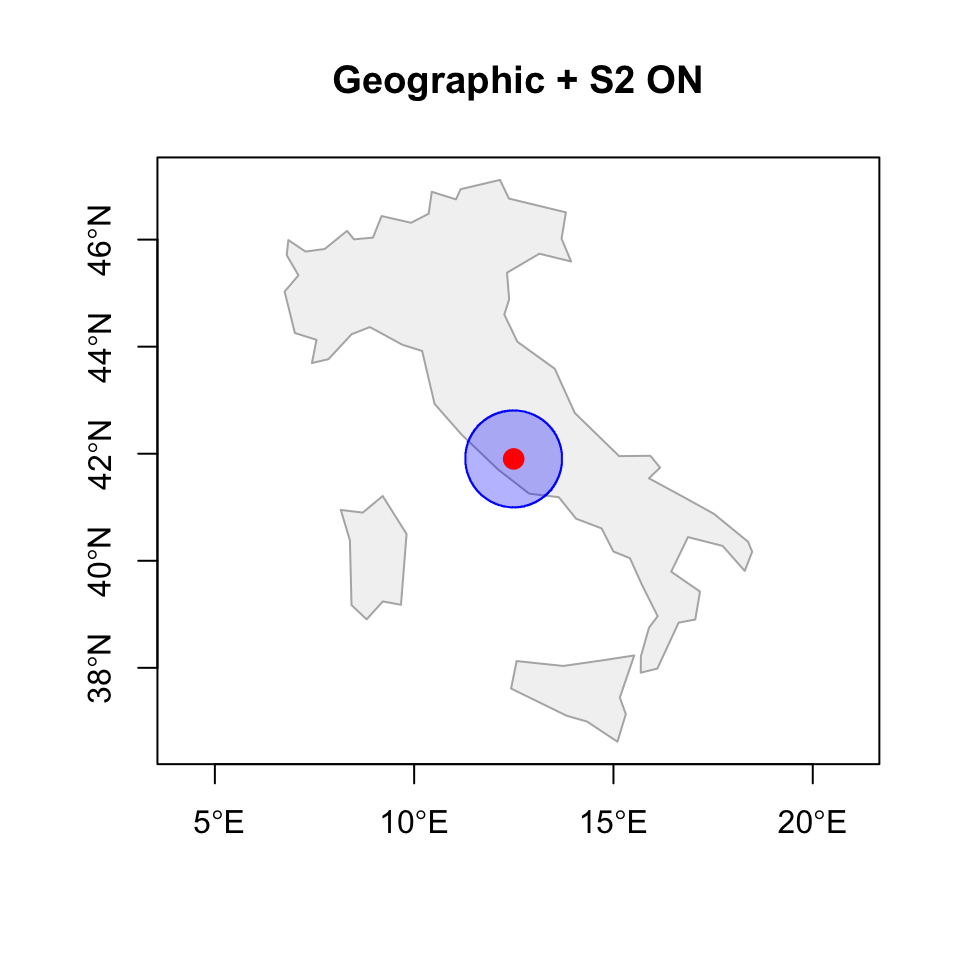
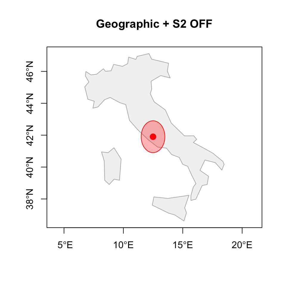
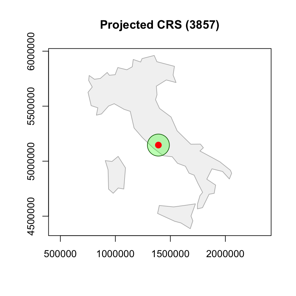
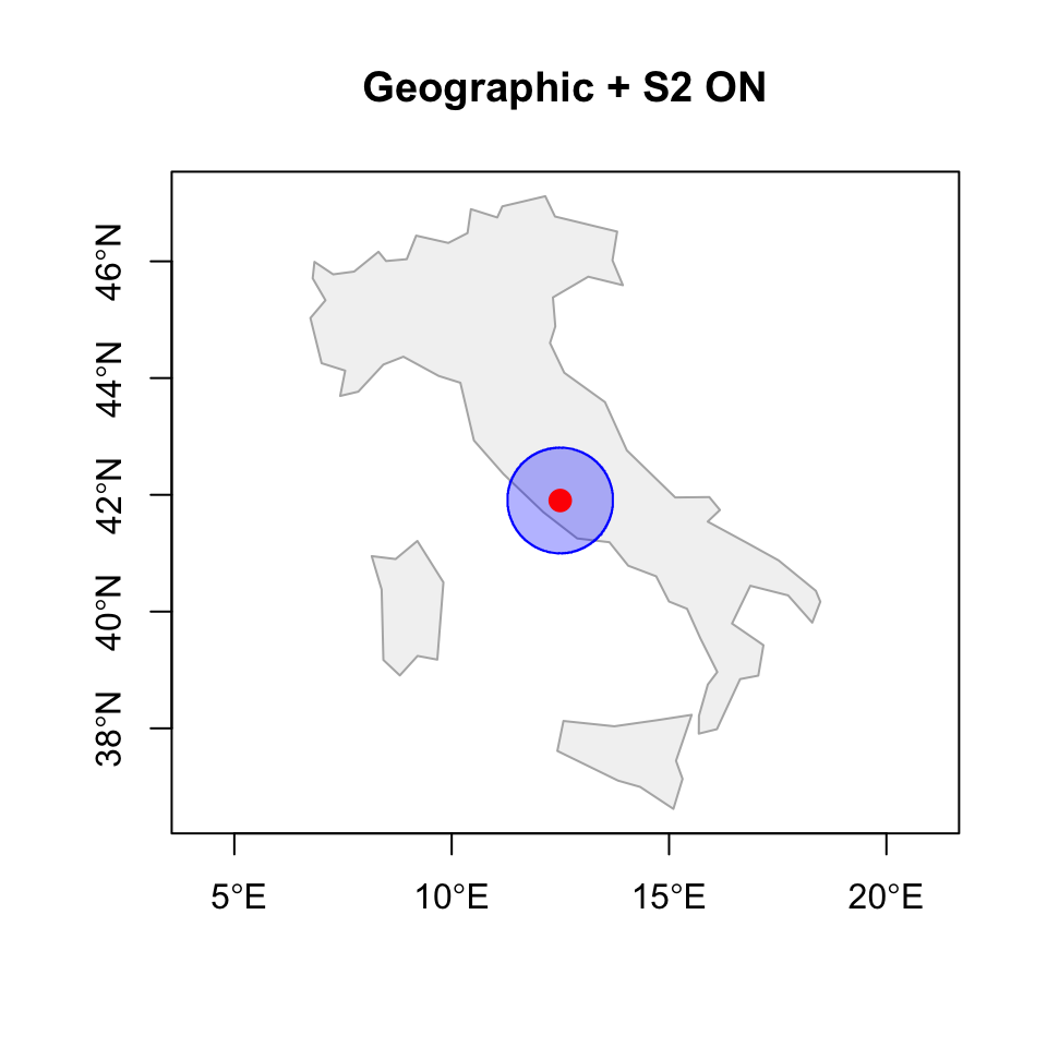
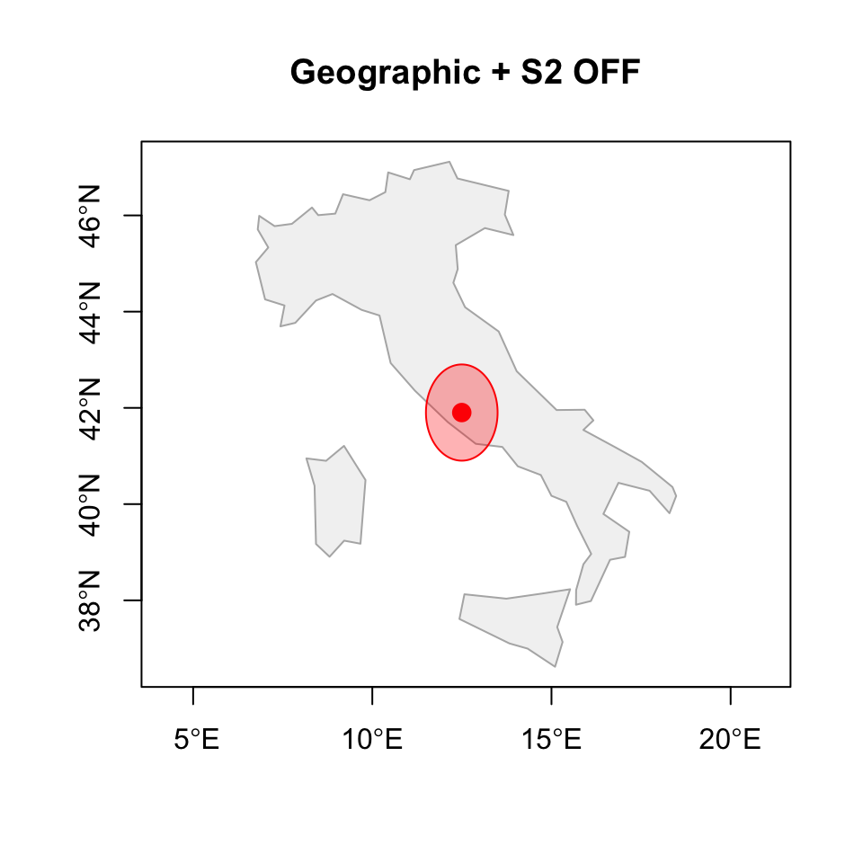
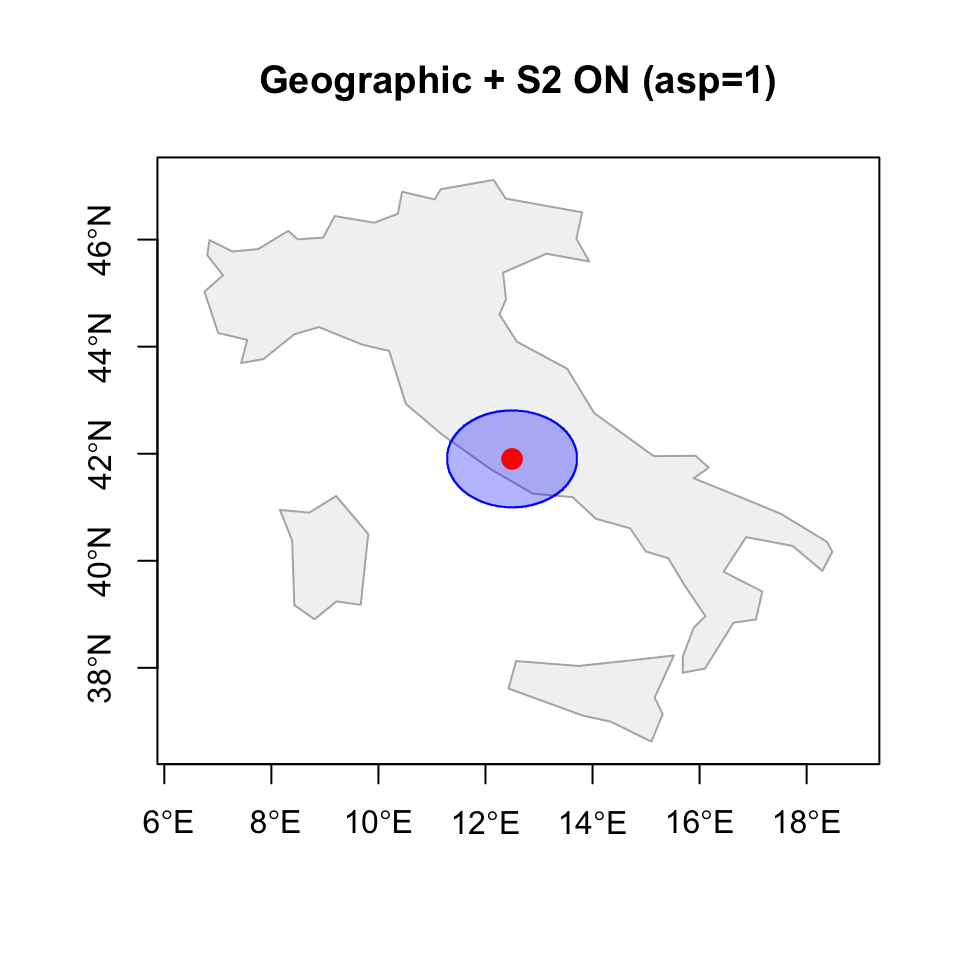
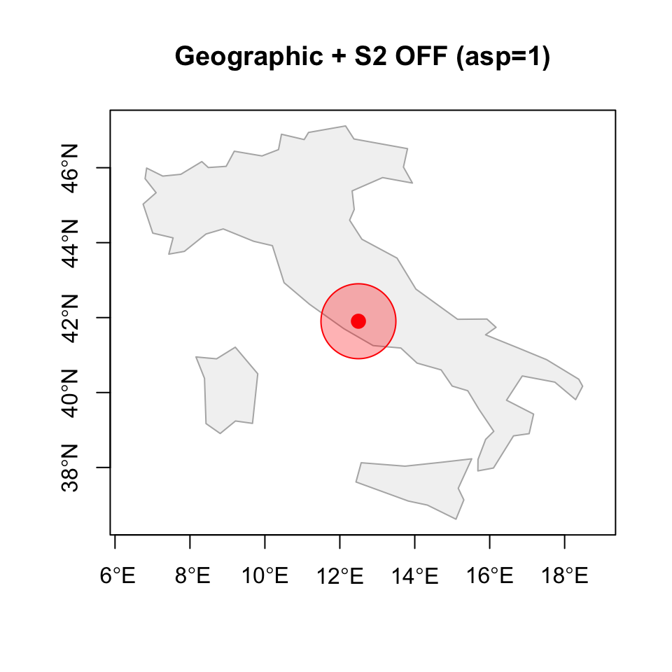
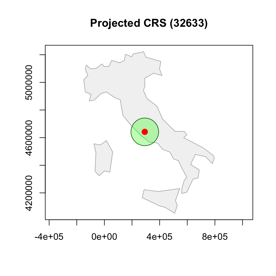
Buffers under different CRS assumptions
italy <- world[world$name_long == "Italy", ]

# S2 ON
sf_use_s2(TRUE)

rome_buffer_s2 <- st_buffer(
  rome_sf,
  dist = 100000
)

# S2 OFF
sf_use_s2(FALSE)

rome_buffer_deg <- st_buffer(
  rome_sf,
  dist = 1 #1 degree!!! using 100000 would be SUPER WRONG!
)

# Back ON
sf_use_s2(TRUE) #useless

# Projected
rome_3857 <- st_transform(rome_sf, 3857)
italy_3857 <- st_transform(italy, 3857)

rome_buffer_proj <- st_buffer(
  rome_3857,
  dist = 100000
)- Why the first one is a circle? Correct km…
- Why the second one is an ellipsoid? It is a cirle in the lon-lat space, but lon-lat are not equal in terms of km…
- Why the third one si smaller? If you’d use a projection specific for Rome, first and third would look much more similar…
Circular on Earth or circular in coordinates?
A common and safe workflow
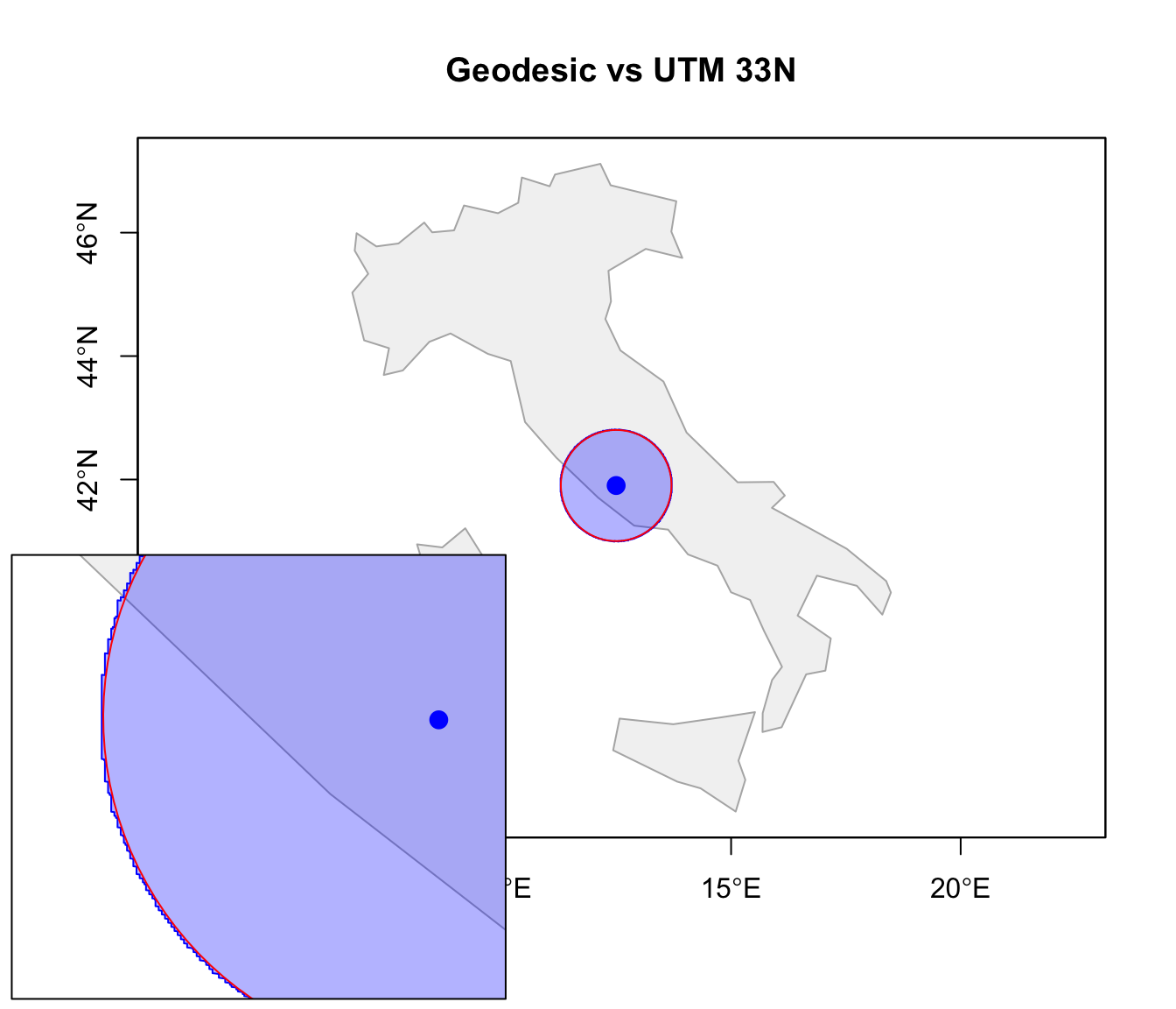
With S2 enabled, many geometry operations work well directly on geographic CRS. However, for local or regional analysis, it is often convenient to:
- start from a geographic CRS (
EPSG:4326); - project the data into a suitable local projected CRS;
- perform geometry operations;
- optionally transform back to WGS84.
rome_32633 <- st_transform(rome_sf, 32633)
# UTM (Universal Transverse Mercator) Zone 33N
# A local projected CRS covering much of Italy.
# Distances are expressed in meters and distortions are very small
# around Rome.

rome_buffer_32633 <- st_buffer(
  rome_32633,
  dist = 100000
)

rome_buffer_wgs84 <- st_transform(
  rome_buffer_32633,
  4326
)
This workflow is especially useful when:
- distances or areas are important;
- the study region is relatively small;
- planar geometry algorithms or GIS libraries assuming Euclidean geometry are used.
Raster data
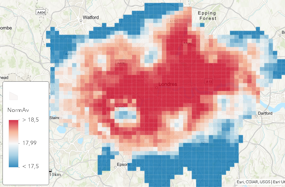
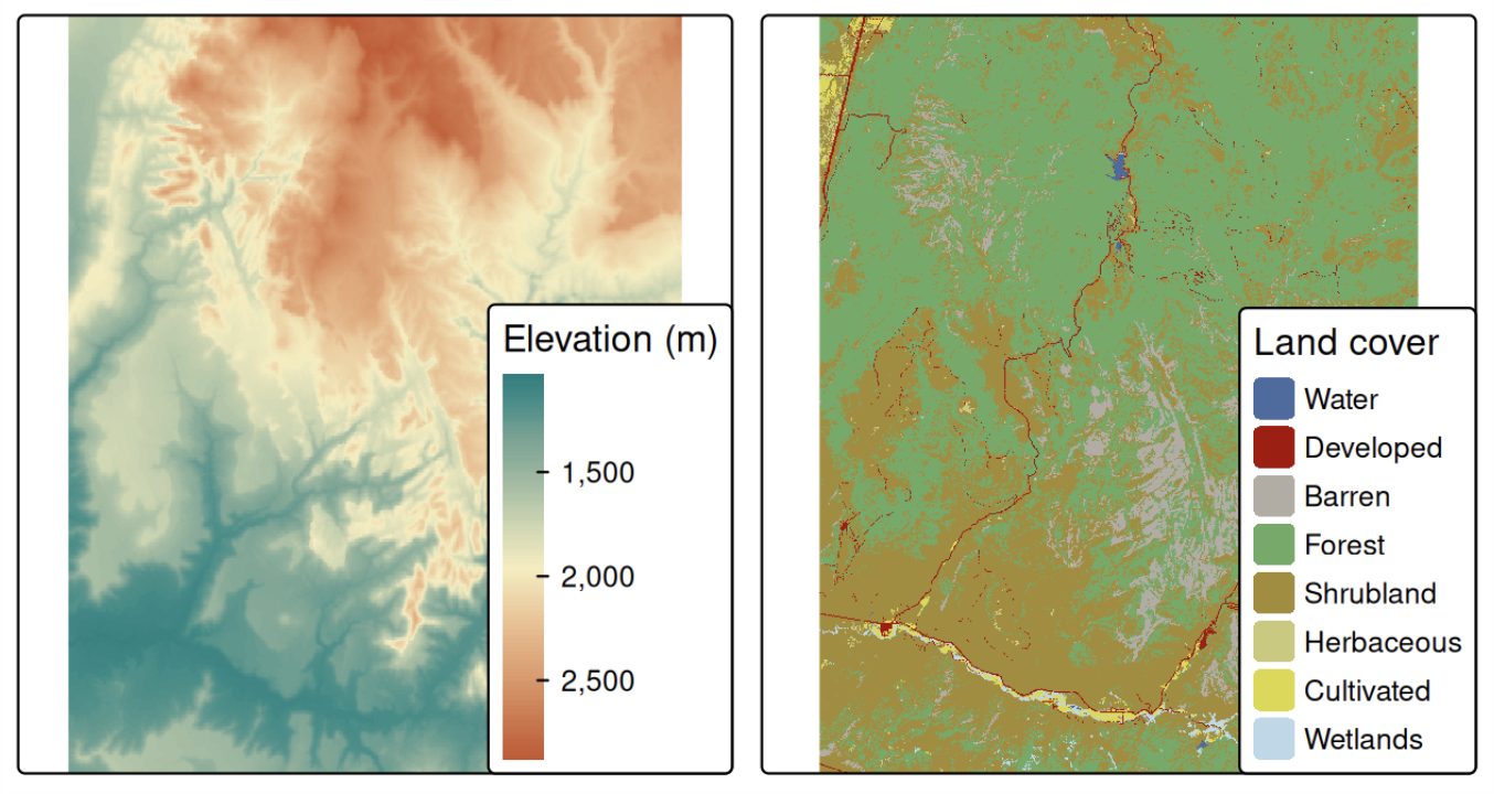
Raster data divide space into a regular grid of cells.
Raster objects can contain:
- a single layer;
- multiple layers (e.g. temperature over time).
Each cell of one raster layer can only hold a single value.
The value might be continuous
- elevation; pollution;
- temperature; precipitation;
- remote sensing variables;
or categorical
- land cover; soil types.
Raster structure
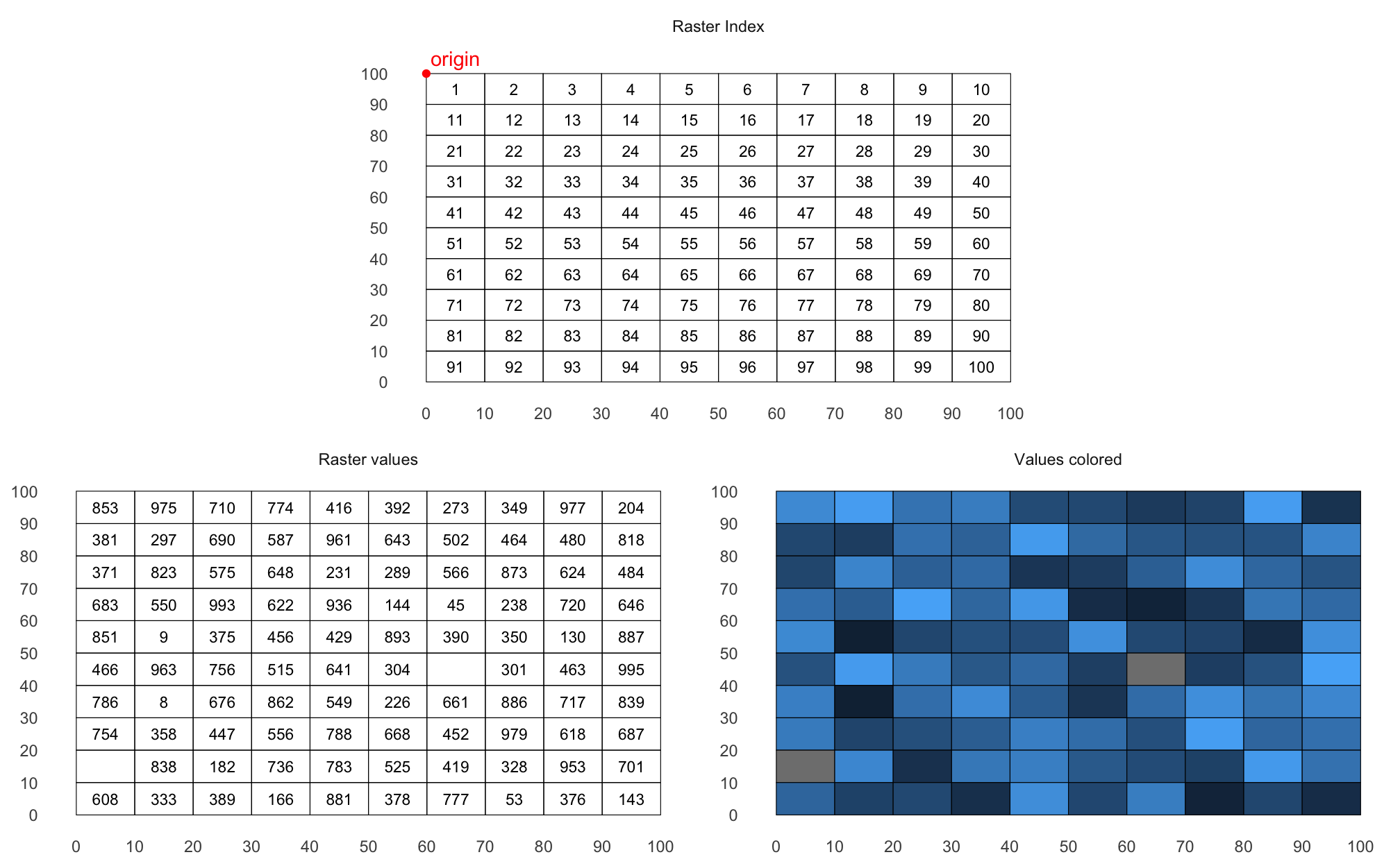
Rasters are fundamentally a matrix of values + spatial metadata.
Unlike vector data, rasters are NOT stored as many polygons: once you know the coordinates of origin (in terra, the upper left corner of the matrix) and the resolution (the amount of space covered by each cell), cell locations are reconstructed.
Plotting and inspecting rasters
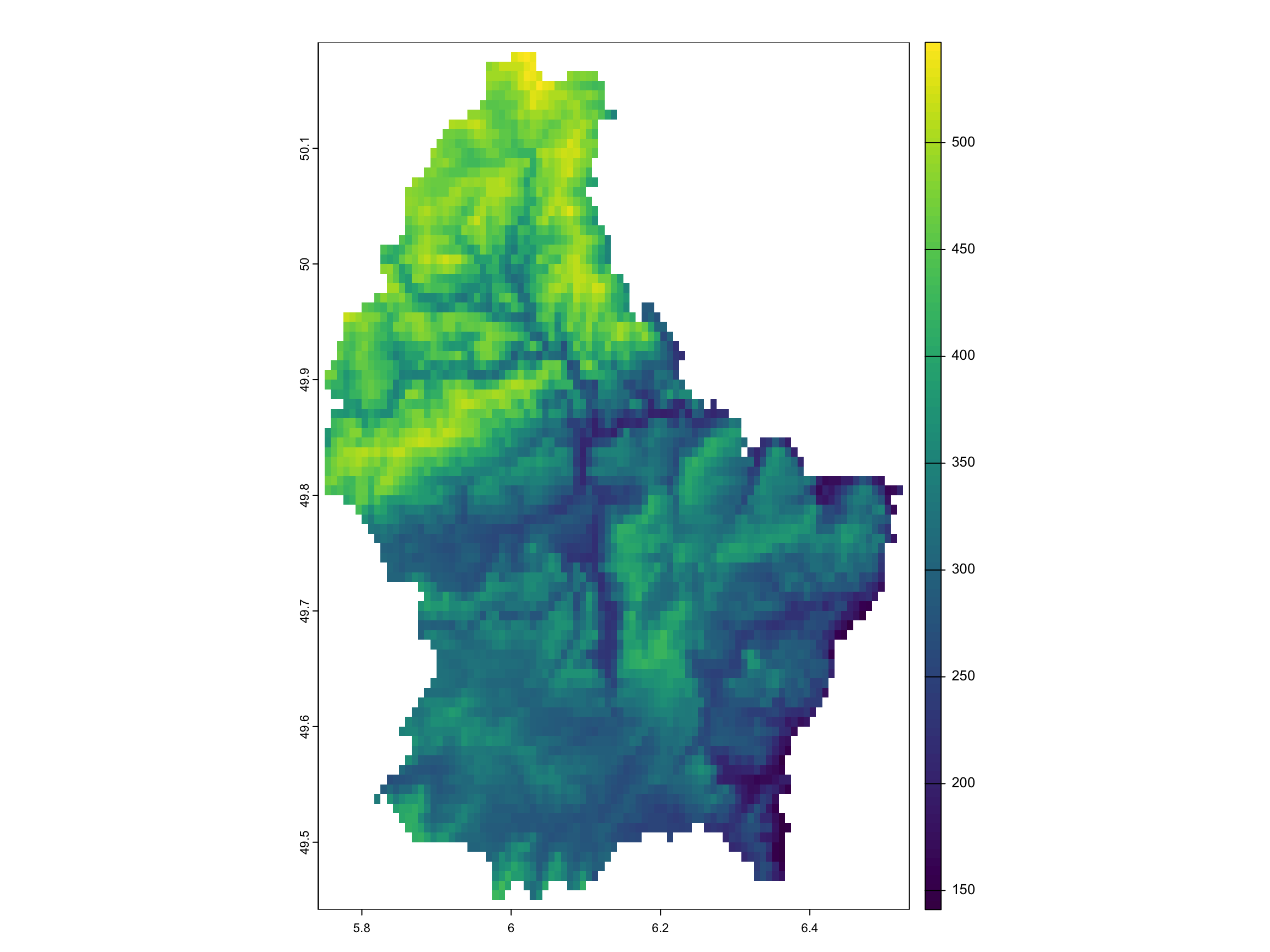
Useful inspection functions include:
Raster matrices are indexed consistently with geographic orientation: columns increase eastward, rows increase southward
Simple math operations are applied cell-by-cell.
Multi-layer rasters
Raster objects can contain multiple aligned layers, each with the same geometry. Each layer stores one value per cell.
class       : SpatRaster
dimensions  : 90, 95, 3  (nrow, ncol, nlyr)
resolution  : 0.008333333, 0.008333333  (x, y)
extent      : 5.741667, 6.533333, 49.44167, 50.19167  (xmin, xmax, ymin, ymax)
coord. ref. : lon/lat WGS 84 (EPSG:4326)
sources     : elev.tif
              memory
              memory
varnames    : elev
              elev
              elev
names       : elevation, elevation, elevation
min values  :       141,       282,       423
max values : 547, 1094, 1641 elevation
1 NA elevation elevation elevation
[1,] NA NA NA
[2,] NA NA NA
[3,] NA NA NA
[4,] NA NA NA
[5,] NA NA NA mean
elevation 348.3366
elevation.1 696.6732
elevation.2 1045.0098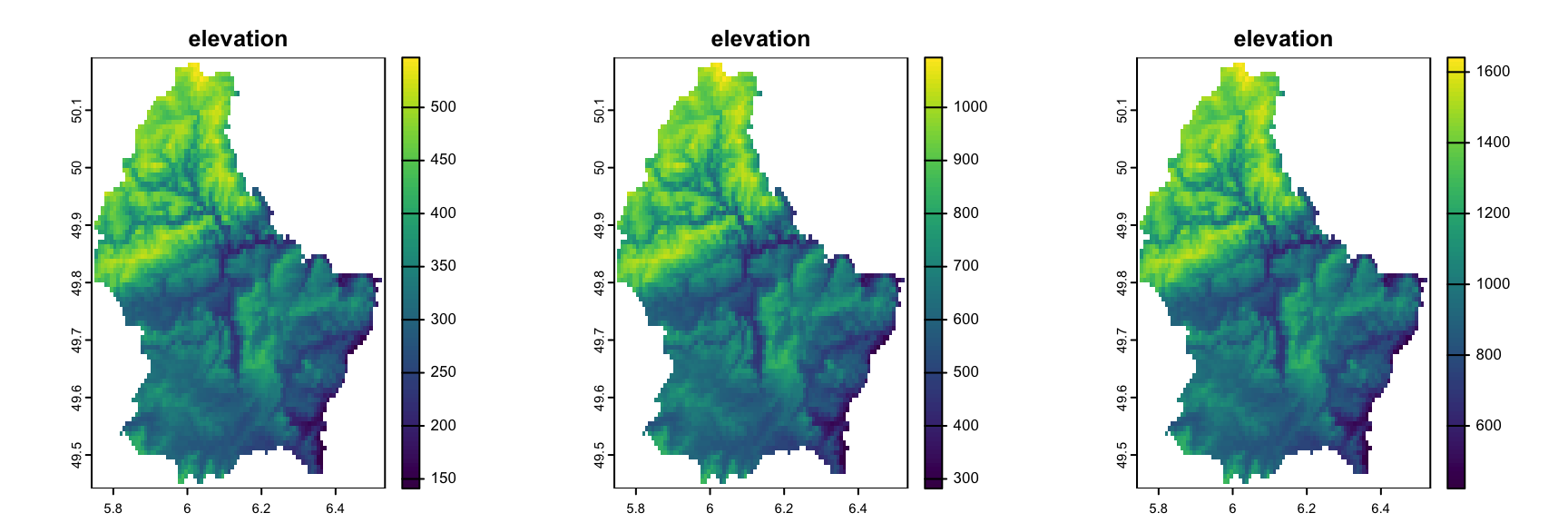
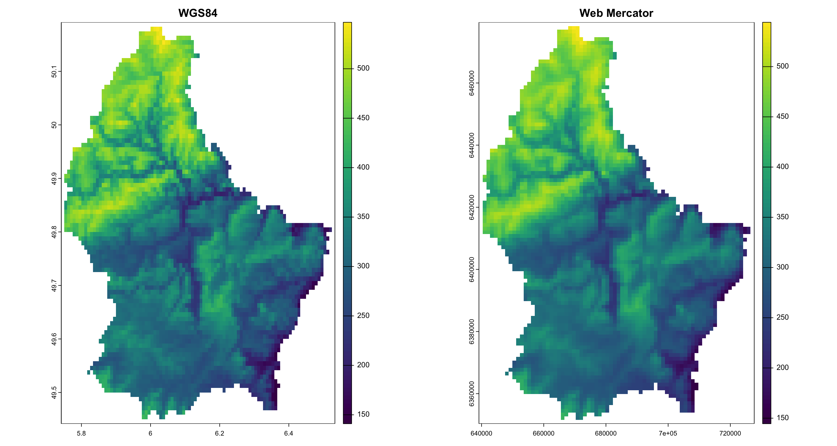
Reprojecting a raster object II
Even visually, you can spot some differences.
Better maps with ggplot
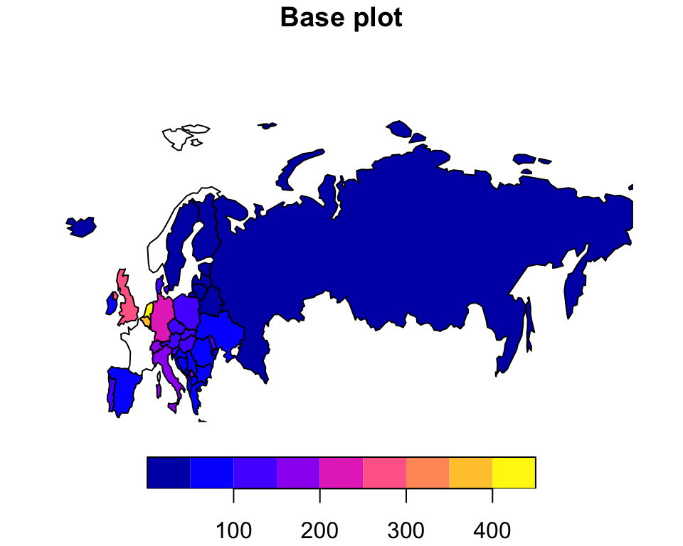
Spatial analysis is also about communicating spatial patterns effectively.
While plot is useful for exploration, ggplot makes much better graphs.
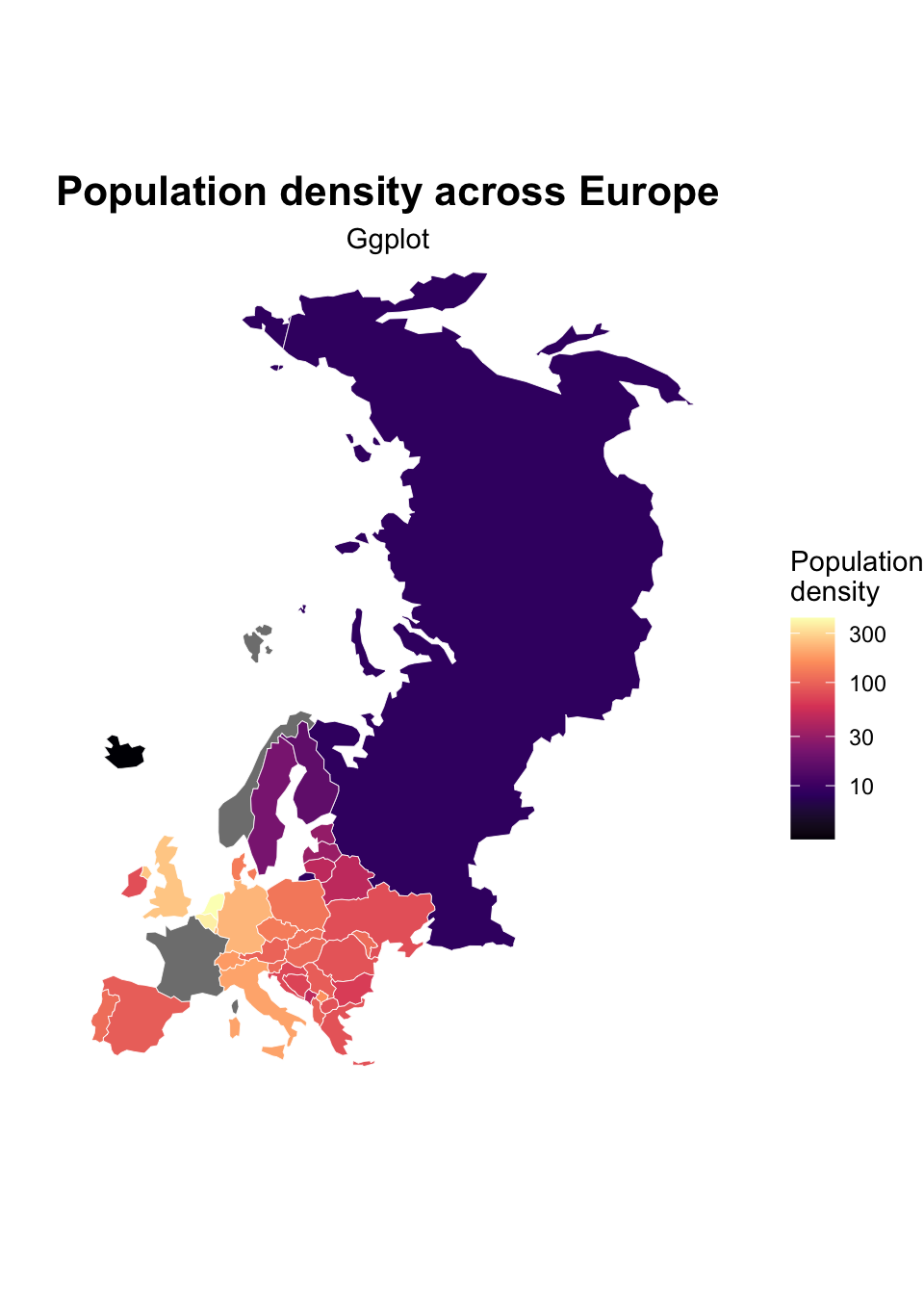
It allows:
- better, more variegated aesthetics;
- layering of multiple spatial objects;
- legends and scales;
- faceting;
- integration with the
tidyverseecosystem; - publication-quality figures.
A first map
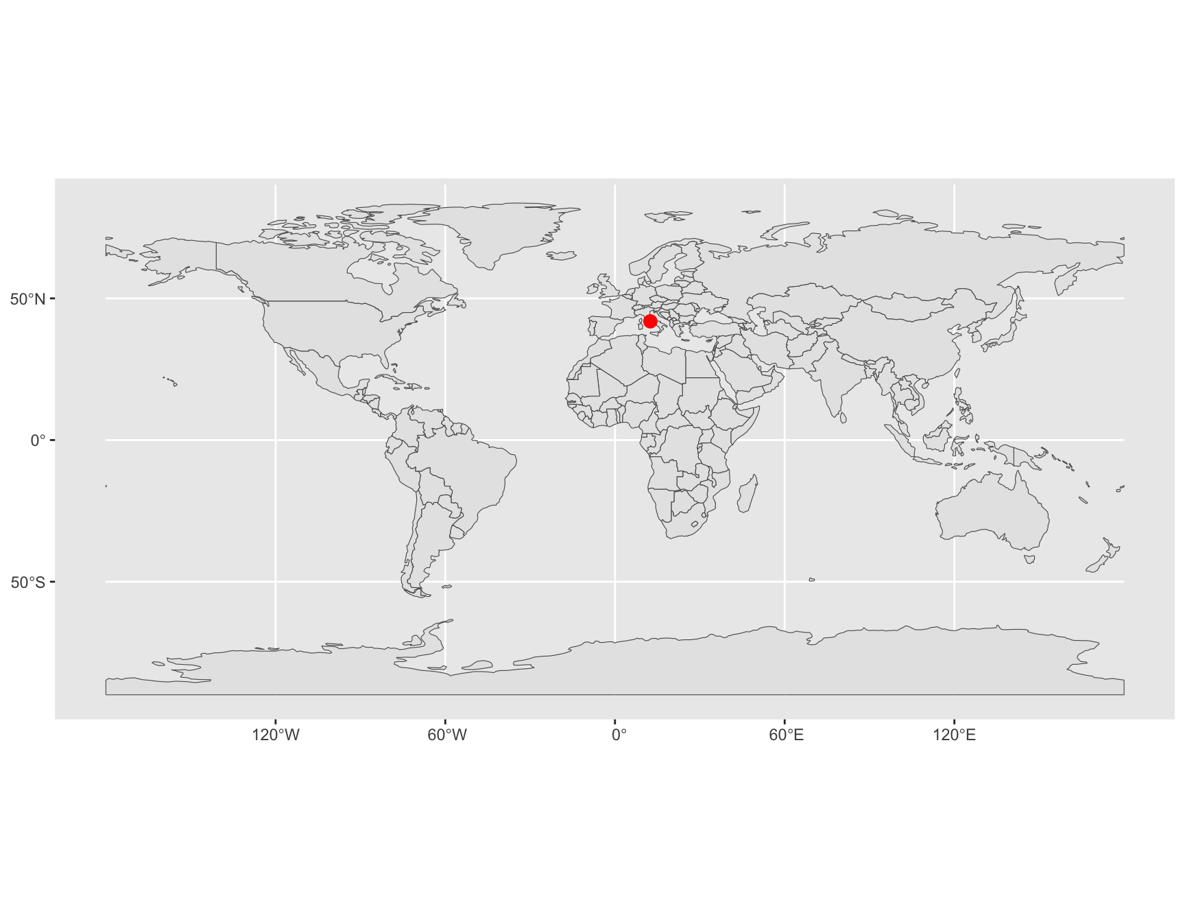
ggplot builds figures by adding layers. For spatial data, the most important layer is geom_sf(), which automatically plots sf objects and handles
- geometries;
- coordinate reference systems;
- map extents.
Layers, vectors and rasters
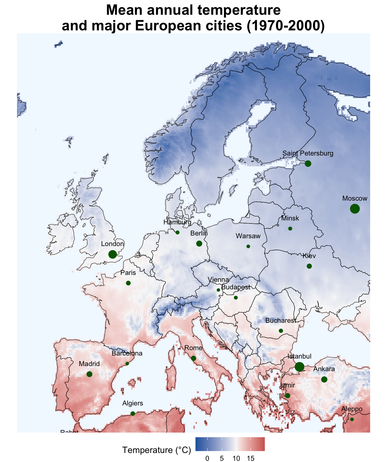
#install packages rnaturalearth, geodata, maps, tidyterra
countries <- rnaturalearth::ne_countries(
  scale = "medium",
  returnclass = "sf"
)

eu <- countries %>%
  filter(region_un%in%c("Europe", "Asia", "Africa"))

tavg <- geodata::worldclim_global(
  var = "tavg",
  res = 10,
  path = tempdir()
)

temp <- mean(tavg)

temp_eu <- crop(
  temp,
  ext(-15, 40, 35, 72)
)

names(temp_eu)

data("world.cities", package = "maps")

cities <- st_as_sf(
  subset(world.cities, pop > 1500000),
  coords = c("long", "lat"),
  crs = 4326
)

cities_lab <- cbind(
  st_drop_geometry(cities),
  st_coordinates(cities)
)

ggplot() +
  tidyterra::geom_spatraster(
    data = temp_eu,
    aes(
      fill = mean
    ),
    alpha = 0.85
  ) +
  geom_sf(
    data = eu,
    fill = NA,
    color = "black",
    linewidth = 0.2
  ) +
  geom_sf(
    data = cities,
    aes(size=pop),
    color = "darkgreen",
    show.legend = FALSE
  ) +
  geom_text(
    data = cities_lab,
    aes(
      X,
      Y,
      label = name
    ),
    size = 3,
    nudge_y = 1
  ) +
  coord_sf(
    xlim = c(-15, 40),
    ylim = c(35, 72),
    expand = FALSE
  ) +
  labs(
    title = "Mean annual temperature and major European cities (1970-2000)"
  ) +
  scale_fill_gradient2(
    low = "#2166AC",
    mid = "#F7F7F7",
    high = "#B2182B",
    midpoint = 10,
    na.value = "aliceblue",
    name = "Temperature (°C)"
  ) +
  theme_void() +
  theme(
    plot.title = element_text(
      face = "bold",
      size = 18,
      hjust = 0.5
    ),
    legend.position = "bottom"
  )