Spatial Data Analysis

Operating with spatial datasets

Sant’Anna School of Advanced Studies

Matteo Coronese
m.coronese@santannapisa.it

June 2026

What will we learn in this course?

Lecture 1 Spatial data basics

Lecture 2 — Operating with spatial datasets

• Who belongs to what? (topological relationships)
• How far is it? (distance relationships)
• What is nearby? (buffers and neighborhoods)
• At which scale do we measure outcomes? (aggregation)
• How to build an exposure measure (raster extraction)

Lecture 3 — Elements of spatial dependence and econometrics

Lecture 4 — Applied spatial workflows

Constructing spatial variables

Spatial variables are rarely directly observed. They are usually constructed from:

• spatial relationships;
• distances;
• overlaps;
• neighboring structures;
• aggregation over space.

Examples:

• distance to the nearest hospital;
• average pollution within a municipality;
• population exposed to flooding;
• neighboring economic activity;
• temperature exposure over agricultural land.

Spatial data manipulation is often aimed at transforming spatial data into measurable, meaningful quantities.

Spatial relationships between geometries

Many spatial variables emerge from relationships between objects. Typical questions include:

• Which points fall inside a polygon?
• Which regions share a border?
• Which observations are within a given distance?
• What is the nearest location?
• Which areas overlap?

Spatial relationships can be conceptually based either on:

Topology

• depends on relative spatial arrangement, independendtly of their distance
• is a binary predicate (TRUE / FALSE)
• is \(x\) inside \(y\)? Does \(x\) overlaps with \(y\)?

Distance:

• depends on physical distance measurements
• mostly continuous, can be binary
• how far is \(x\) w.r.t \(y\)? Is \(x\) within 100km w.r.t \(y\)?

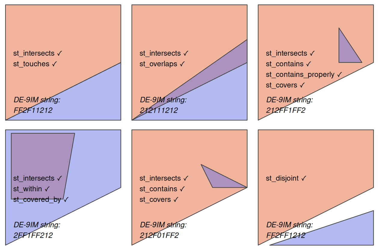
Topological relationships

• Binary topological relationships are qualitative, logical statements (TRUE / FALSE).

• They form the theoretical basis for spatial joins (merging data based on their spatial relations).

• Order is important!

  • e.g. equals, intersects, crosses, touches and overlaps are symmetrical
  • e.g. contains and within are not

• Topological relationships do not require meaningful distance units.

Their formal mathematical definition can be quite complex. We will instead focus on the sf functions that implement them.

Simple topological relations

st_intersects() is a catch-all predicate, identifying cases of touch, cross or within. Examples:

• which cities belong to which countries;
• which regions overlap;
• which observations fall inside a buffer.

polygon_matrix <- cbind(
  x = c(0, 0, 1, 1,   0),
  y = c(0, 1, 1, 0.5, 0)
)
polygon_sfc <- st_sfc(st_polygon(list(polygon_matrix)))
#we could have created an sf object. 
#This is just to show you that sf commants works also
#without attributes, as long as they have a geometry

point_df <- data.frame(
  x = c(0.2, 0.7, 0.4),
  y = c(0.1, 0.2, 0.8)
)
point_sf <- st_as_sf(point_df, coords = c("x", "y"))

• Topological predicates often return sparse lists of spatial relationships.

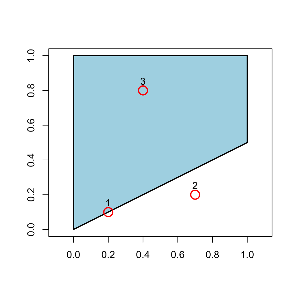
int <- st_intersects(point_sf, polygon_sfc) 
int

Sparse geometry binary predicate list of length 3, where the predicate
was `intersects'
 1: 1
 2: (empty)
 3: 1

class(int) #sgbp object

[1] "sgbp" "list"

length(int) #1 list of lenght 3 (1 polygon, 3 points)

[1] 3

int[[1]] 

[1] 1

#tells you whether point 1 intersects 
#with which polygon (in this case, number 1)

Simple topological relations II

It might be more convenient to have a non-sparse output

int_nsp <- st_intersects(point_sf, polygon_sfc, sparse=FALSE)
int_nsp

      [,1]
[1,]  TRUE
[2,] FALSE
[3,]  TRUE

class(int_nsp) #matrix object

[1] "matrix" "array" 

dim(int_nsp)# 1 column, 3 rows (1 polygon, 3 points)

[1] 3 1

int_nsp[2,1] #is point 2 intersecting with polygon number 1? 

[1] FALSE

The same logic applies to other predicates: Which points are within the polygon?

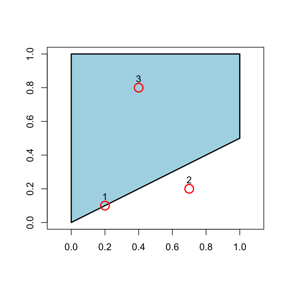
st_within(point_sf, polygon_sfc, sparse=FALSE)

      [,1]
[1,] FALSE
[2,] FALSE
[3,]  TRUE

Which points touch the polygon?

st_touches(point_sf, polygon_sfc, sparse=FALSE)

      [,1]
[1,]  TRUE
[2,] FALSE
[3,] FALSE

Which points are disjoint (the opposite of intersect?)

st_disjoint(point_sf, polygon_sfc, sparse=FALSE)

      [,1]
[1,] FALSE
[2,]  TRUE
[3,] FALSE

A concrete example - To which province each city belongs to?

Topological relations \(\rightarrow\) Question: what belongs to what?

• Which labour market area contains each firm?
• Which protected area contains each habitat?
• Which flood zone contains each building?
• Which households are covered by a mobile network?

prov <- giscoR::gisco_get_nuts(
  year = "2021",
  nuts_level = 3,
  country = "IT",
  resolution = "01"
)

regions <- giscoR::gisco_get_nuts(
  year = "2021",
  nuts_level = 2,
  country = "IT",
  resolution = "01"
) %>%
  st_drop_geometry() %>%
  select(
    region_id = NUTS_ID,
    region_name = NUTS_NAME
  )

prov %<>%
  mutate(
    region_id = substr(NUTS_ID, 1, 4)
  ) %>% 
  left_join(.,
            regions,
            by="region_id")

prov %<>% select(NUTS_NAME, region_name)

data("world.cities", package = "maps")

cities <- world.cities %>% 
  filter(country.etc=="Italy")

cities <- st_as_sf(
  cities,
  coords = c("long", "lat"),
  crs = 4326
)

Then

ct_int <- st_intersects(
  cities,
  prov
)

The output is still a sparse list: for each city, we obtain the province(s) it intersects.

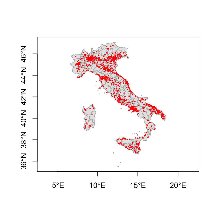
ct_int[[6]] #city number 6 is located in province 33

[1] 8

st_drop_geometry(cities[6, ])

              name country.etc   pop capital
6 Aci Sant'Antonio       Italy 17566       0

st_drop_geometry(prov[33,"NUTS_NAME"])

   NUTS_NAME
33    Arezzo

table(lengths(ct_int)) 

  0   1 
 27 958 

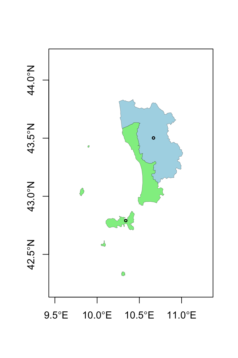
All cities are matched at most with one province, which makes sense. But wait, how can it be that we also have zeros?

Spatial data are messy :)

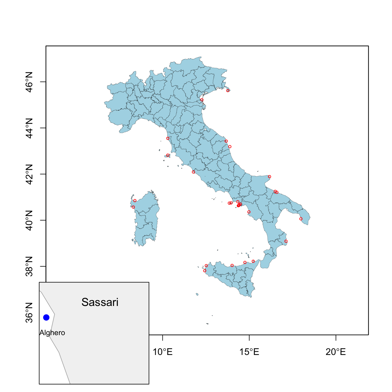
missing <- cities[lengths(ct_int) == 0, ]

missing$name #resolution matters!

All of them are coastal cities

• Resolution matters!
• Topological relationships are not always enough. We are going to need distances to fix them.

Spatial joins

The output of st_intersects() contains all the information we need:

ct_int_sp <- st_intersects(
  cities,
  prov,
  sparse = FALSE
)

Each row refers to a city, each column to a province.

dim(ct_int_sp) #985 rows, one per each city

[1] 985 107

#107 columns, one per each province

st_drop_geometry(cities[6,])

              name country.etc   pop capital
6 Aci Sant'Antonio       Italy 17566       0

st_drop_geometry(prov[which(ct_int_sp[6, ]),"NUTS_NAME"])

  NUTS_NAME
8   Catania

We could manually use this information to transfer province attributes:

prov_id <- apply(
  ct_int_sp,
  1,
  function(x){
    w <- which(x)
    if(length(w) == 1) w else NA
  }
)
cities$province <- prov$NUTS_NAME[prov_id]
st_drop_geometry(cities[1:5,])

           name country.etc   pop capital province
1   Abano Terme       Italy 19167       0   Padova
2 Abbiategrasso       Italy 30515       0   Milano
3        Acerra       Italy 51394       0   Napoli
4  Aci Castello       Italy 17930       0  Catania
5    Aci Catena       Italy 28459       0  Catania

Spatial joins II

Spatial joins automate exactly this process:

cities_prov <- st_join(
  cities,
  prov
)
st_drop_geometry(cities_prov[1:5,c("name","NUTS_NAME")])

           name NUTS_NAME
1   Abano Terme    Padova
2 Abbiategrasso    Milano
3        Acerra    Napoli
4  Aci Castello   Catania
5    Aci Catena   Catania

A spatial join is analogous to a database join, except that the matching key is a spatial relationship rather than a common identifier.

By default:

st_join(cities, prov, join = st_intersects)

but other predicates can also be used:

st_join(..., join = st_within)
st_join(..., join = st_contains)
st_join(..., join = st_touches)

By default st_join performs a left join. left=FALSE operates a inner join.

A similar logic governs spatial subsetting, which uses st_intersect as default

pisa <- prov %>% filter(NUTS_NAME == "Pisa")
cities[pisa,]

                     name country.etc   pop capital province
188               Cascina       Italy 40959       0     Pisa
207 Castelfranco di Sotto       Italy 11990       0     Pisa
660                  Pisa       Italy 87401       0     Pisa

Note that if you inspect cities_prov, you will find some NA in the province column: coastal problematic cities prevent a proper join.

Distance relationships

Topological relationships tell us whether two objects are spatially related. Many empirical questions require more information:

Distance relations \(\rightarrow\) Question: What can people, firms, or regions reach?

• Healthcare accessibility (e.g nearest hospital);
• Access to labour markets (e.g. distance to major employment centers);
• Exposure to environmental hazards (e.g. distance from coast, rivers, pollution centers);
• Market access and trade costs (e.g. distance from ports, infrastructures);

The main function you need to use is st_distance().

Distances depend on the coordinate system.

Recall from Lecture 1:

• geographic CRS (e.g. WGS84) store coordinates;
• projected CRS (e.g. UTM) store locations in planar units;
• distances are meaningful only when the units themselves are meaningful.

rome <- cities %>%
  filter(name == "Rome")

milan <- cities %>%
  filter(name == "Milan")

st_distance(
  rome,
  milan
)

Units: [m]
         [,1]
[1,] 479684.8

Distance and coordinate systems

The same distance can be computed using different representations of the Earth.

st_distance(rome, milan)

Units: [m]
         [,1]
[1,] 479684.8

sf_use_s2(FALSE)

st_distance(rome, milan)

Units: [m]
         [,1]
[1,] 479820.7

sf_use_s2(TRUE) #turn it on again 

cities_32632 <- st_transform(
  cities,
  32632
)

st_distance(
  cities_32632[cities_32632$name=="Rome",],
  cities_32632[cities_32632$name=="Milan",]
)

Units: [m]
         [,1]
[1,] 479803.6

Unlike st_buffer, distances are generally safe in geographic coordinates. Without S2, the geodetic (shortest distance between to points on the surface of Earth) you are computing is even slightly more accurate.

All three approaches hey rely on different geometric assumptions:

• S2 ON: spherical Earth;
• S2 OFF: ellipsoidal Earth;
• UTM: planar approximation.

For Rome–Milan (~480 km), the discrepancy is only about 100 meters.

Pairwise distances

st_distance() can compute distances between many geometries at once.

d <- st_distance(
  cities[1:5, ]
)
rownames(d) <- cities$name[1:5]
colnames(d) <- cities$name[1:5]

The result is a distance matrix.

Rows and columns correspond to spatial observations. In this case, we are computing all pair-wise distances between 5 specific cities.

n geometries × n geometries \(\rightarrow\) n × n distance matrix

You can also pass two distinct vectors:

d2 <- st_distance(
  cities[1:5, ],
  cities[6:9, ]
)
rownames(d2) <- cities$name[1:5]
colnames(d2) <- cities$name[6:9]

n geometries × m geometries \(\rightarrow\) n × m distance matrix

Distance matrices are the building blocks of many spatial methods:

• distance-based exposure measures;
• spatial weights matrices;
• spatial econometrics;
• Conley standard errors.

Point-to-polygon distances

So far we have computed distances between points. When a polygon is involved, the distance is computed w.r.t. the nearest edge.

Some cities could not be assigned to a province because of geometry resolution issues. Instead of asking:

Which province contains this city?

we can ask:

Which province is closest to this city?

agropoli <- missing[1, ]

d <- st_distance(
  agropoli,
  prov
)

prov$NUTS_NAME[which.min(d)]

[1] "Salerno"

This identifies the nearest province using distances.

st_nearest_feature() automates this process.

st_nearest_feature(
  missing,
  prov
)

 [1] 58 90 45 74 27 65 76 96 49 27 27 14 27 70  3 74 44 98 27 16 18 90 70 27  3
[26] 27 43

The result is the index of the closest province for each city.

We can now fix the NA is cities

missing_prov <- st_join(
  missing,
  prov,
  join = st_nearest_feature
)

cities_prov_fixed <- bind_rows(
  cities_prov %>% 
    filter(!is.na(NUTS_NAME)),
  missing_prov
)

Distances between polygons

What happens when two or more polygons are involved?

pisa <- prov %>%
  filter(NUTS_NAME == "Pisa")

livorno <- prov %>%
  filter(NUTS_NAME == "Livorno")

st_distance(
  pisa,
  livorno
)

Units: [m]
     [,1]
[1,]    0

Why? st_distance computes the minimum distance, and Pisa and Livorno (!) share a border.

A distance of zero may be perfectly reasonable:

• neighboring municipalities;
• adjacent administrative regions;
• contiguous land parcels.

However, many social science applications require representing each area by a single location:

• commuting between municipalities;
• trade between regions; gravity models.
• spatial spillovers.

st_centroid(pisa) #returns the geometrical center of a polygon
st_point_on_surface(livorno) #sometimes the centroid falls out 
#of the polygon... or even in the sea

Geometry-derived variables and neighborhoods

Geometries can generate new variables.

prov %>% 
  mutate(
    area = st_area(geometry)
  ) %>% st_drop_geometry() %>% slice(1:5)

  NUTS_NAME region_name             area
1   Treviso      Veneto 2471738729 [m^2]
2     Nuoro    Sardegna 5636855056 [m^2]
3   Trapani     Sicilia 2460671584 [m^2]
4    Padova      Veneto 2112795108 [m^2]
5    Rovigo      Veneto 1664049154 [m^2]

Areas can be useful:

• to normalize measures which increase with land (e.g. # storms);
• compute e.g. population density; agricultural land share, GDP per km^2

Buffers define local neighborhoods around geometries.

rome_buffer <- st_buffer(
  st_transform(rome, 32632),
  50000
) %>% 
  mutate(is_close_rome = TRUE)

The buffer contains all locations within 50 km of Rome.

Buffers can be used to construct distance-based relationships (when proximity matters!)

cities_utm <- st_transform(
  cities,
  32632
) #remember our lecture on projections

st_join(
  cities_utm,
  rome_buffer %>% select(is_close_rome),
  join = st_intersects
) %>% filter(is_close_rome) %>% 
  st_drop_geometry() %>% slice(1:4)

                name country.etc   pop capital province is_close_rome
1     Albano Laziale       Italy 37278       0     Roma          TRUE
2 Anguillara Sabazia       Italy 17666       0     Roma          TRUE
3              Anzio       Italy 49354       0     Roma          TRUE
4            Aprilia       Italy 66871       0   Latina          TRUE

#The join identifies all cities located within the buffer. 
#This is equivalent to asking: Which cities are within 50 km of Rome? 

A shorthand is st_is_within_distance.

Examples:

• assigning households to the nearest hospital;
• assigning firms to the nearest port;
• identifying municipalities within 50 km of a power plant;
• measuring population exposed to a flood event.

Spatial aggregation

Spatial data often come at a finer resolution than the one needed for analysis.

Suppose we want to estimate the population of each Italian province from city-level data.

cities_prov_fixed #geometry = city points

To obtain province-level geometries, we replace city geometries with province polygons

cities_prov_new <- cities_prov_fixed %>%
  st_drop_geometry() %>%
  left_join(
    prov %>% select(NUTS_NAME, geometry),
    by = "NUTS_NAME"
  ) %>%
  st_as_sf()

nrow(cities_prov_new)

[1] 985

So far, only ordinary tabular join. Question: could have we obtained the same with st_join?

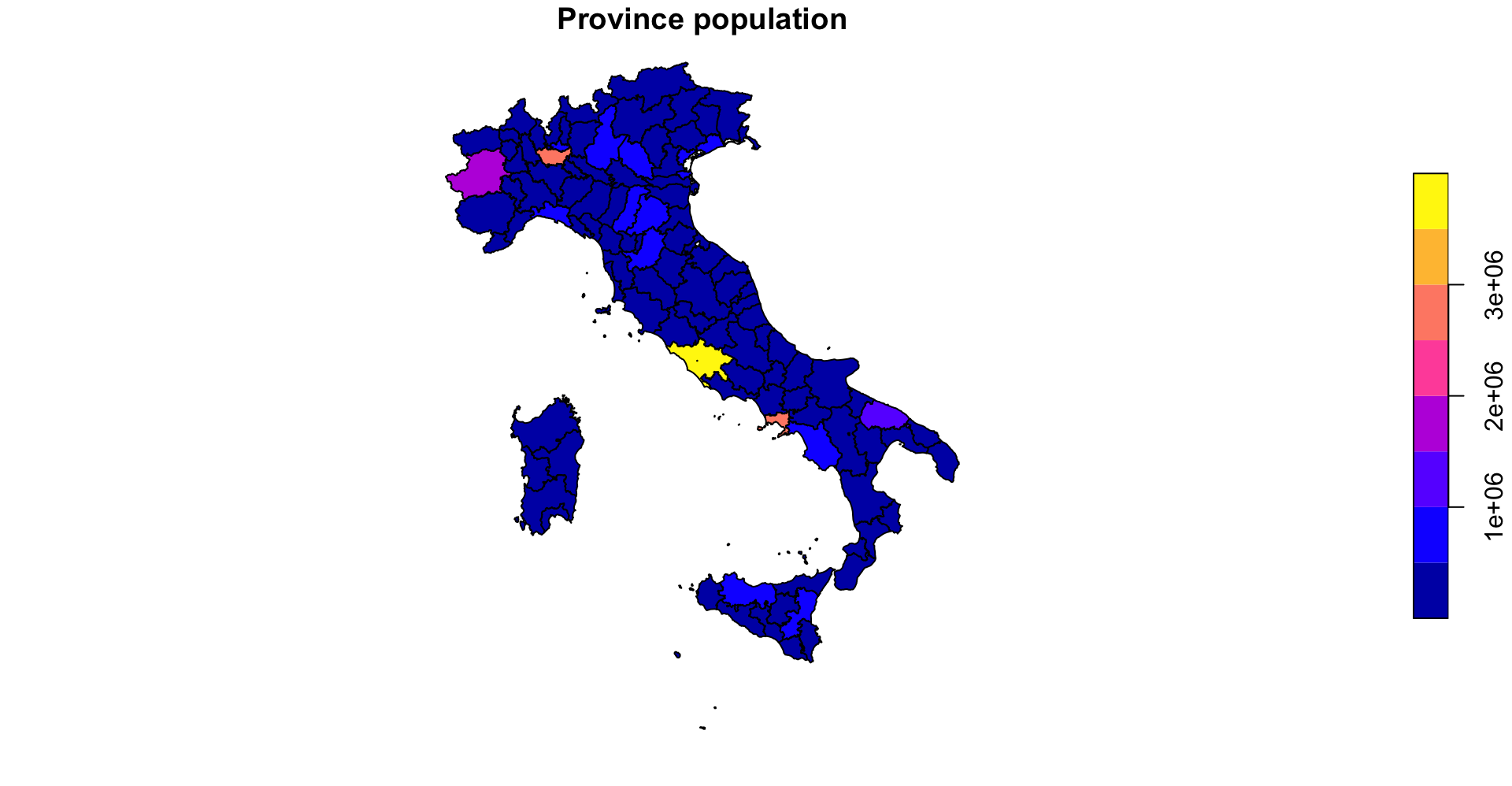
The aggregation sums population across all cities belonging to the same province.

prov_pop <- cities_prov_new %>%
  group_by(NUTS_NAME) %>%
  summarise(
    pop = sum(pop),
    region_name= first(region_name)
  ) 

nrow(prov_pop)

[1] 107

The resulting dataset contains one observation per province.

Spatial aggregation II

We can further aggregate provinces into regions.

reg_pop <- prov_pop %>%
  group_by(region_name) %>%
  summarise(
    pop = sum(pop)
  )

The population of each region is obtained by summing provincial populations.

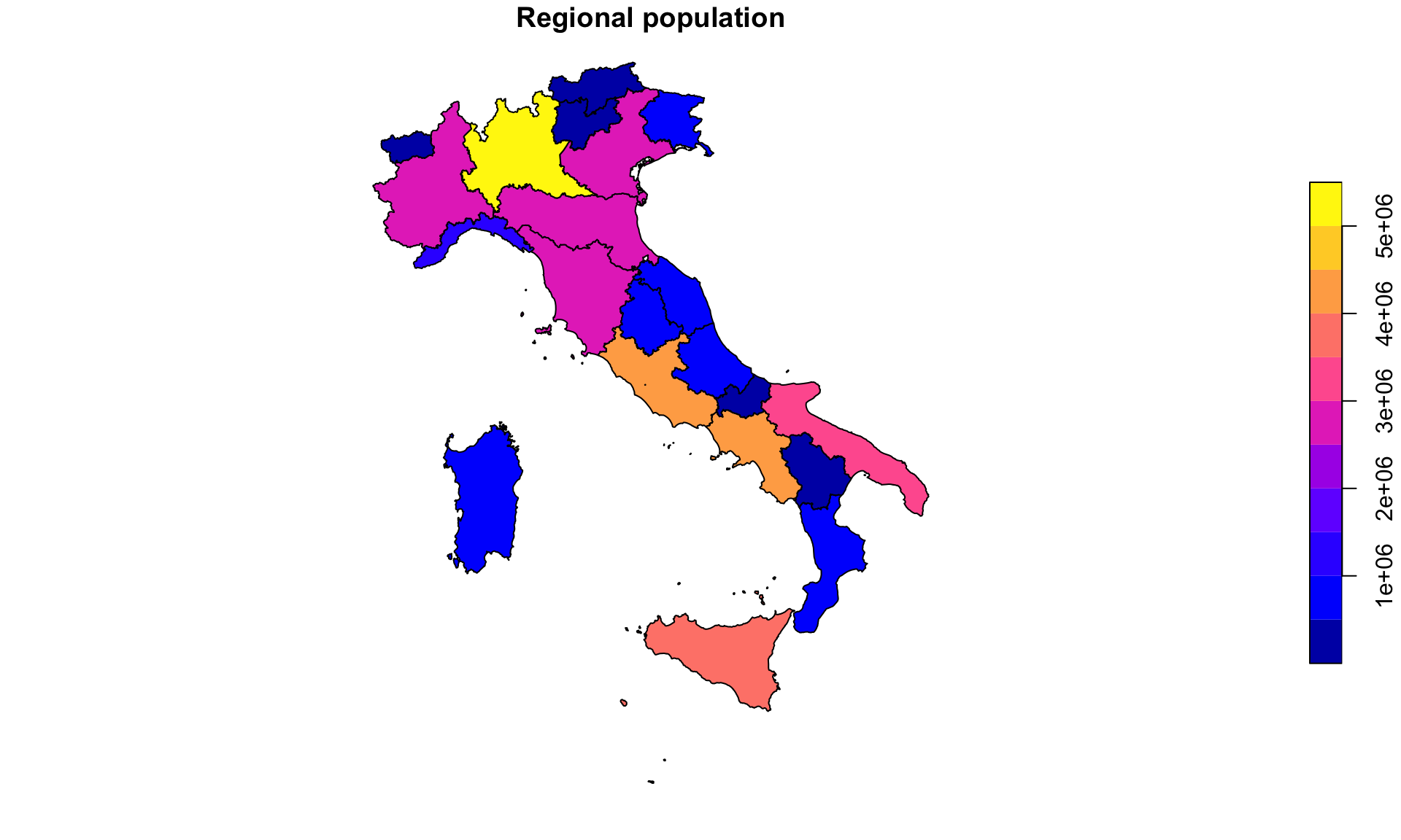
nrow(prov_pop)

[1] 107

nrow(reg_pop)

[1] 21

107 provinces
↓
21 regions

• Spatial aggregation: unlike ordinary data frames, summarise() also automatically aggregates geometries.sf performs a geometric union (st_union()).

Question: wich is the right scale of analysis?

• Construct regional indicators from local data;

  • Labour: firms → labour market areas; workers → commuting zones
  • Environment: pollution or climate observations → administrative units
  • Urban: crime incidents, traffic accidents, Airbnb listings → census tracts
  • Telecom: signal measurements, mobile-phone pings → coverage areas

• Harmonize data at different administrative scales;

Raster-vector interactions

Practical research often requires raster-vector interaction.

Question: What is the average temperature of each Italian province?

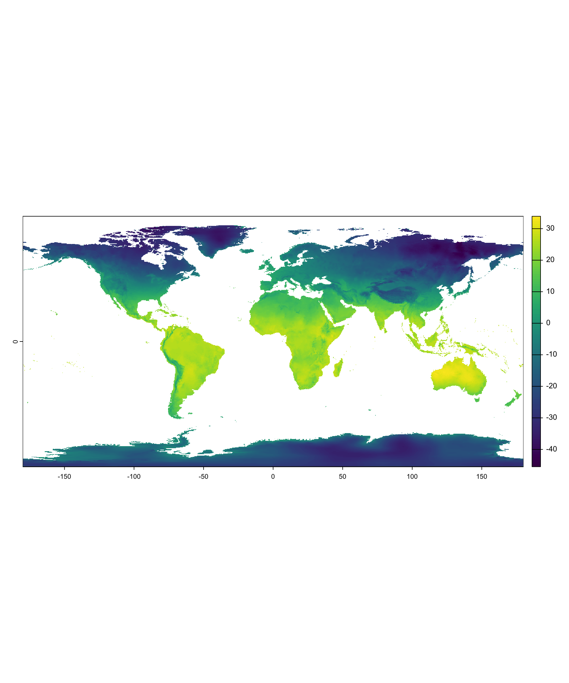
We have climate information as a raster. Our provinces are polygons. How do we combine them?

Similar questions:

• Population exposed to high pollution
• Vegetation conditions (NDVI) around farms;
• Night-time lights as a proxy for local economic activity;
• Heat exposure of workers across labour market areas;

library(terra)

tavg <- geodata::worldclim_global(
  var = "tavg",
  res = 5, #minutes of degree
  path = tempdir()
)

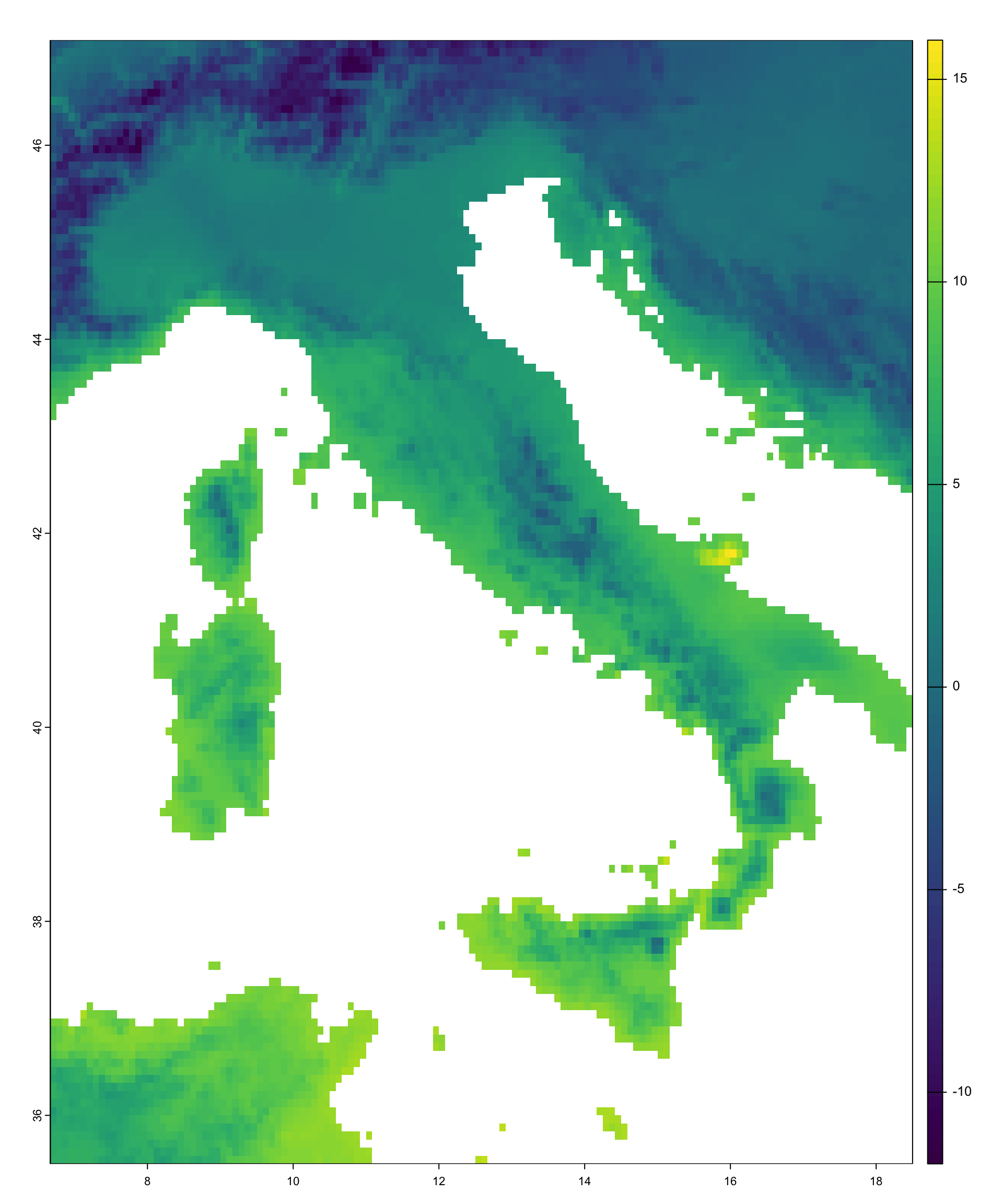
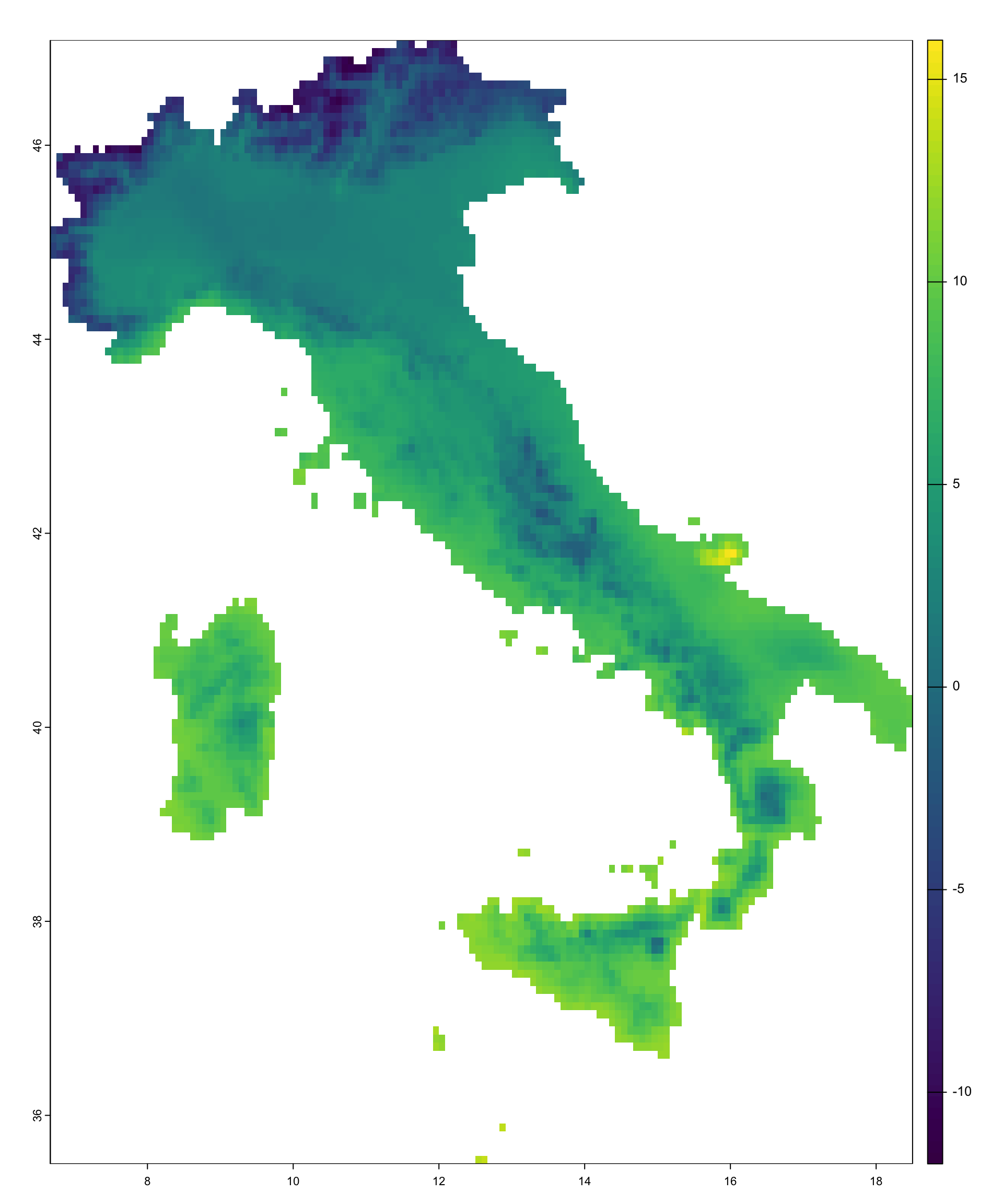
#A global raster contains to much information than we need
italy <- prov %>%
  summarise()

tavg_crop <- crop(tavg, italy) 
#restricts the raster extent (using the bbbox): focus on Italy

tavg_it <- mask(tavg_crop,italy)
#removes cells outside Italy (using the center of the cell)

Raster extraction

Raster extraction transfers raster information to vector geometries, by means of an aggregating function.

temp_prov <- terra::extract(
  tavg_it, #we are using all layers
  prov,
  fun = mean,
  na.rm = TRUE
)

head(temp_prov[,3],3)

[1]  4.005000  7.718002 10.910698

prov <- cbind(prov, temp_prov[,-1])

names(prov)

 [1] "NUTS_NAME"        "region_name"      "wc2.1_5m_tavg_01" "wc2.1_5m_tavg_02"
 [5] "wc2.1_5m_tavg_03" "wc2.1_5m_tavg_04" "wc2.1_5m_tavg_05" "wc2.1_5m_tavg_06"
 [9] "wc2.1_5m_tavg_07" "wc2.1_5m_tavg_08" "wc2.1_5m_tavg_09" "wc2.1_5m_tavg_10"
[13] "wc2.1_5m_tavg_11" "wc2.1_5m_tavg_12" "geometry"        

prov <- prov %>% #fancy renaming
  rename_with(
    ~ paste0("temp_", tolower(month.abb)),
    contains("tavg")
  )

The result is nlyr new variables attached to each province.

Local, focal, zonal, global. Raster extraction can be interpreted as a form of zonal aggregation. The zones are defined by vector geometries rather than by another raster.

Raster cells
      ↓
Province polygons
      ↓
Mean temperature

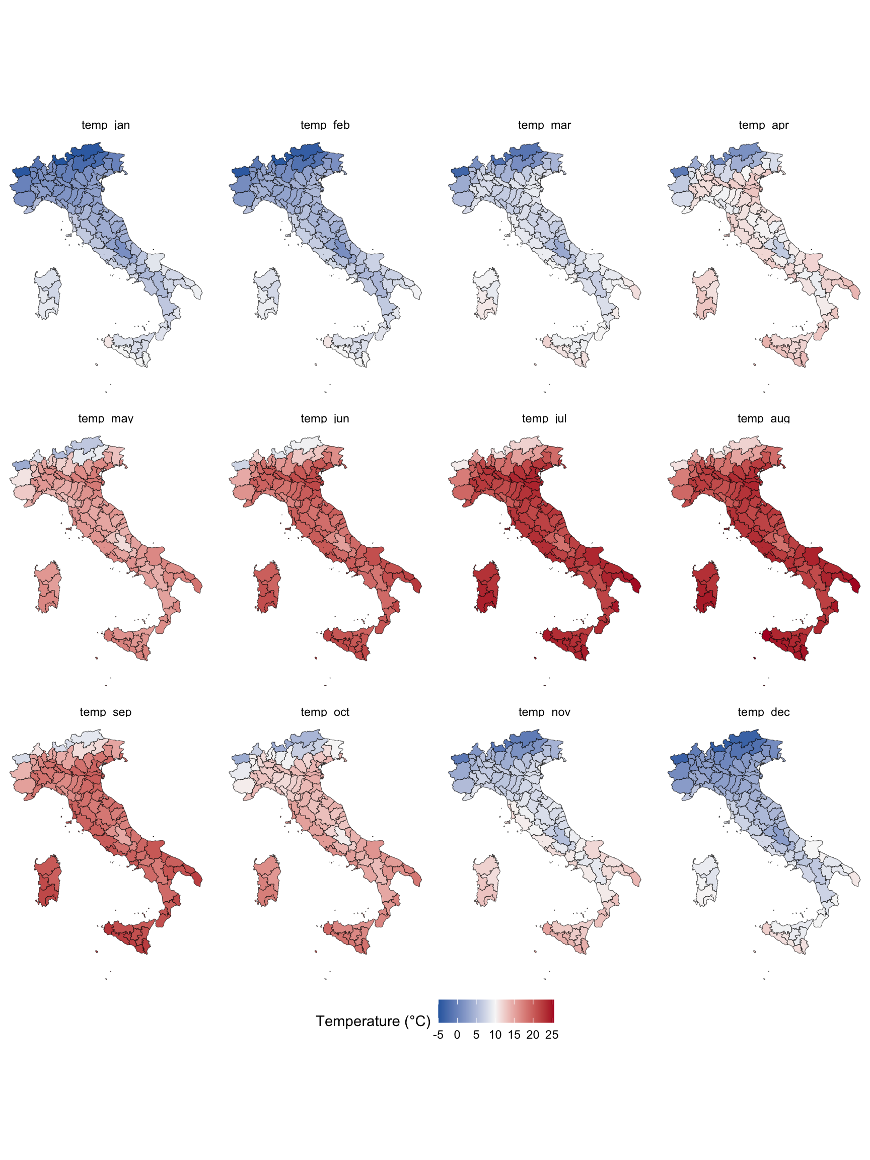
Question:

Which month do you expect to display the strongest North–South gradient?

A nice plot

prov %>%
  pivot_longer(
    cols = starts_with("temp_"),
    names_to = "month",
    values_to = "temperature"
  ) %>% 
  mutate(
    month = factor(
      month,
      levels = paste0(
        "temp_",
        c("jan","feb","mar","apr","may","jun",
          "jul","aug","sep","oct","nov","dec")
      )
    )
  ) %>% 
  ggplot() + 
  geom_sf(aes(fill=temperature))+ 
  facet_wrap(month~., nrow=2) +
  scale_fill_gradient2(
    low = "#2166AC",
    mid = "#F7F7F7",
    high = "#B2182B",
    midpoint = 10,
    na.value = "aliceblue",
    name = "Temperature (°C)"
  ) + 
  theme_void() +
  theme(
    legend.position = "bottom"
  )

Exact extraction (Lecture 4 teaser)

Standard extraction treats raster cells as fully inside or outside a polygon.

+-----------------------+
|                       |
|         60%           |
|        outside        |
|                       |
|   Province boundary   |
──────────────────────────
|                       |
|         40%           |
|        inside         |
|                       |
+-----------------------+

What should we do with this cell?

• Ignore it?
• Keep the whole cell?
• Use only the fraction that falls inside the province?

Weighted extraction accounts for partial overlaps.

#install.packages("exactextractr")
exactextractr::exact_extract(
  tavg_it,
  prov,
  fun="mean"
)

Each raster cell contributes proportionally to the area intersecting the polygon.

This is particularly important when:

• raster resolution is coarse;
• polygons are small;
• more generally, when the #cell/polygon area is small

We will return to this issue in Lecture 4.