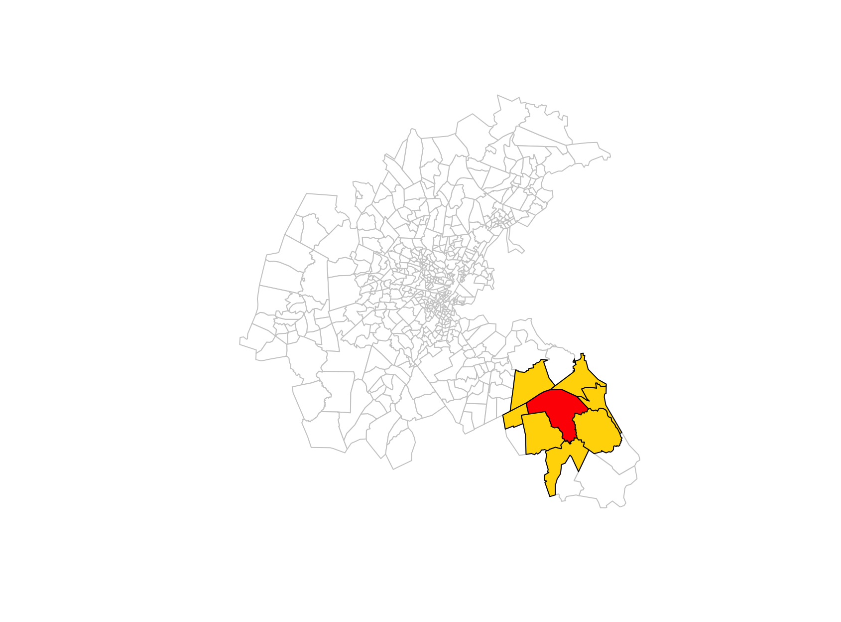
Spatial Data Analysis

Elements of spatial dependence and econometrics

Sant’Anna School of Advanced Studies

Matteo Coronese
m.coronese@santannapisa.it

June 2026

What will we learn in this course?

Lecture 1 Spatial data basics

Lecture 2 — Operating with spatial datasets

Lecture 3 — Elements of spatial dependence and econometrics

• Spatial dependence and OLS assumptions
• Variograms and Conley standard errors
• Spatial weights matrices and spatial lags
• Moran’s I and LISA
• SLX, SAR and SEM models

Lecture 4 — Applied spatial workflows

Is space a problem?

“Everything is related to everything else, but near things are more related than distant things.”

• Tobler’s First Law of Geography

Space is not only a data format. It is a source of dependence that affects both prediction and causal inference:

• Air pollution crosses administrative borders;
• Labour markets extend beyond municipalities;
• Housing prices spill over across neighborhoods;
• Temperature shocks affect nearby regions simultaneously.

As a consequence, observations located close in space are often not independent.

Spatial dependence arises when observations are statistically dependent across space because of interactions, spillovers, or shared environments.

Spatial dependence and OLS

Consider the standard linear model:

\[ \mathbf{y} = \beta\mathbf{X} + \mathbf{\varepsilon} \]

Key assumptions underlying OLS estimation and inference:

\[ 1) \quad E[\varepsilon_i \varepsilon_j] = 0 \qquad i \neq j \] Errors are uncorrelated across observations.

\[ 2) \quad E[\mathbf{\varepsilon} | \mathbf{X}] = 0 \] Exogeneity: regressors are uncorrelated with the errors.

Spatial dependence creates two distinct problems:

1. Inference problem
   • Nearby units share common shocks \(\rightarrow\) assumption 1) fails.
   • Consequence: inefficient estimates, incorrect standard error.
2. Modeling problem
   • Spatial spillovers or interactions are relevant but omitted \(\rightarrow\) assumption 2) fails.
   • Consequence: biased and inconsistent estimates.

Different methods address these problems differently.

Dealing with spatial dependence

Different models encode different assumptions about how space operates:

• Conley SE: robust inference (more agnostic)
• SEM: model error dependence
• SLX: model covariate spillovers
• SAR: model outcome spillovers

The distinction is useful pedagogically, but in practice different mechanisms often coexist. You often need theory to distinguish among the various alternatives.

                      Spatial dependence
                              │
                              ▼
                   What mechanism generates
                     spatial dependence?
                              │
           ┌──────────────────┴──────────────────┐
           │                                     │
           ▼                                     ▼
   Correlated errors                   Spatial interactions
    Cov(εᵢ, εⱼ) ≠ 0                        are omitted
           │                                E[ε|X] ≠ 0 
           │                                     │
      Need robust                         What interacts?
    inference only?                              │
           │                                     │
           │                                     │
      ┌────┴────┐                         ┌──────┴──────┐
      │         │                         │             │
      ▼         ▼                         ▼             ▼
     Yes       No                    Neighboring   Neighboring
      │         │                     covariates    outcomes
      │         │                         │             │
      ▼         ▼                         ▼             ▼
   Conley      SEM                       SLX           SAR

What generates spatial dependence?

Suppose we study the effect of temperature on income:

\[ Income_i = \beta Temp_i + \varepsilon_i \]

• Spatial correlation in income may indicate spatial dependence.
• Spatial correlation in temperature is not a problem per se.

The key question is: Does spatial dependence remain after conditioning on observed covariates?

        Spatial clustering in income
                     ↓
      Temperature may explain part of it
                     ↓
        Estimate OLS: Income ~ Temp
                     ↓
  Do income still cluster after conditioning 
on temperature (i.e. do residual still cluster?)
                     │
            ┌────────┴────────┐
            │                 │
           No                Yes
            │                 │
       Observed X     Unexplained spatial
      accounts for    dependence remains
     the clustering           │
                              ▼
                       Spatial methods

Different mechanisms might explain spatial correlation. A heatwave arrive in Pisa:

Mechanism	Pisa–Livorno example	Consequence
Shared shocks	Pisa and Livorno share unobserved regional factors	(Cov(\(\varepsilon_i\),\(\varepsilon_j\))\(\neq0\))
Covariate spillovers	Workers commute: temperature in Pisa affects income in Livorno	Omitted neighboring covariates → endogeneity \((E[\varepsilon|X]\neq0)\)
Outcome spillovers	Lower income in Pisa affects economic activity in Livorno	Omitted neighboring outcome → simultaneity \((E[\varepsilon|X]\neq0)\)

Spotting spatial dependence: variograms

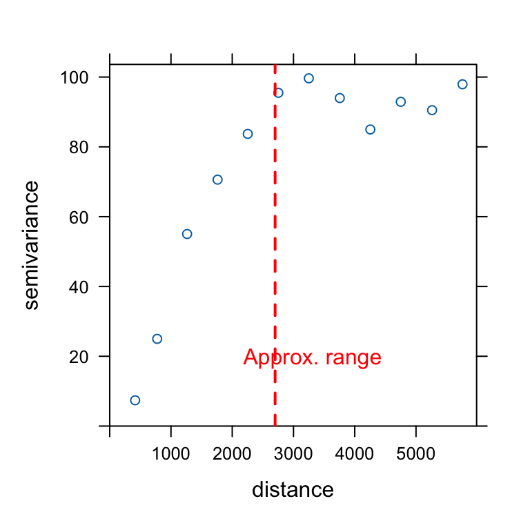
A variogram describes how the dissimilarity (semi-variance) between observations changes with distance. The variogram does not require a pre-specified spatial structure: it directly relies on pairwise distances between observations.

\[ \text{Semivariance} \quad \gamma(h) = \frac{1}{2N(h)} \sum_{(i,j)\in h} (Z_i-Z_j)^2 \]

• \(Z_i\) and \(Z_j\) are the values observed in regions \(i\) and \(j\);
• \(N(h)\) is the number of pairs of obs separated by distance (\(h\)).

The variogram is obtained by computing the semivariance for increasing distance classes (binning, e.g. 0–50 km, 50–100 km, etc.).

boston.tr <- st_read(system.file("shapes/boston_tracts.gpkg", package = "spData"))

boston_utm <- boston.tr %>% st_transform(., 32619) #utm19N
boston <- st_transform(boston_utm, 4326)
boston_utm_pts <- st_centroid(boston_utm)
vg <- variogram(MEDV ~ 1, 
                data = boston_utm_pts, 
                cutoff = 6000,
                width = 500)

plot(vg)

• Low semivariance: observations are similar.
• High semivariance: observations are more different.
• Plateau (sill): beyond this point, increasing distance adds little information.

• Scale: semivariance is scale-variant: the plateau often approximate total variance (hence the \(1/2\)).
• Range: distance beyond which spatial dependence becomes negligible.

Spatial dependence after OLS

We estimate a simple hedonic model of housing prices:

\[ MEDV_i = \beta_0 + \beta_1 CRIM_i + \beta_2 RM_i + \beta_3 NOX_i + \beta_4 LSTAT_i + \varepsilon_i \]

where:

• MEDV is the median housing value in the census tract;
• CRIM is the per-capita crime rate;
• RM is the average number of rooms per dwelling;
• NOX measures air pollution concentration;
• LSTAT is the share of socioeconomically disadvantaged population.

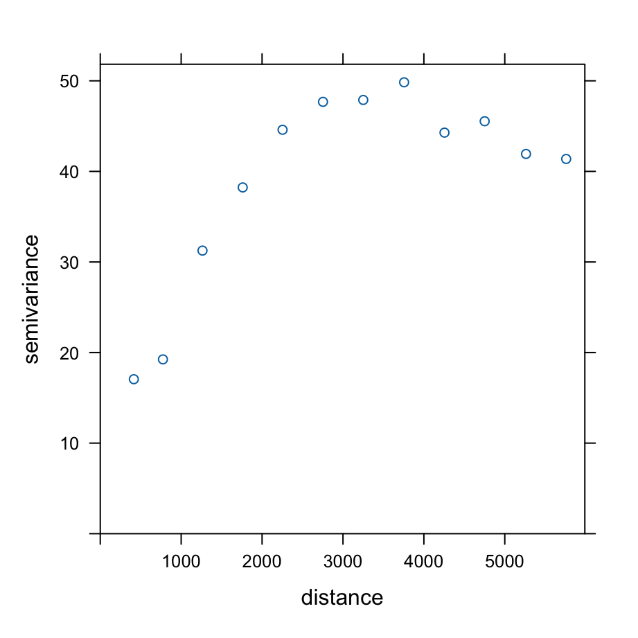
We then compute the variogram of the OLS residuals. Residual semivariance remains lower at short distances.

Spatial dependence may persist even after controlling for observable characteristics, potentially violating the OLS assumption of independent errors.

m <- lm(
  MEDV ~ CRIM + RM + NOX + LSTAT,
  data = boston_utm_pts
)

boston_utm$resid <- resid(m)

vg_res <- variogram(
  resid ~ 1,
  data = boston_utm,
  cutoff = 6000,
  width = 500
)

plot(vg_res)

Spatially robust inference: Conley standard errors

Spatially correlated residuals violate the OLS assumption of independent errors:

\[ E[\varepsilon_i \varepsilon_j] = 0 \qquad i \neq j \]

Conley standard errors relax this assumption by allowing residual correlation to decay with geographic distance.

Idea: Nearby observations may share common shocks, while observations beyond a chosen cutoff distance are assumed independent.

Importantly, Conley does not modify coefficient estimates. Only the estimated uncertainty changes:

\[ \hat{\beta}_{Conley} = \hat{\beta}_{OLS} \qquad SE_{Conley} \neq SE_{OLS} \] In this example, we use a 2 km cutoff, consistent with the range suggested by the residual variogram.

library(fixest)

coords <- st_coordinates(st_centroid(boston))

boston$lon <- coords[,1]
boston$lat <- coords[,2]


mf <- feols(
  MEDV ~ CRIM + RM + NOX + LSTAT,
  data = boston
)

summary(
  mf,
  vcov = vcov_conley(cutoff = 2.5,
                lat = "lat",
                lon = "lon")
)

                                 mf                mf.1
Dependent Var.:                MEDV                MEDV
                                                       
Constant             -2.519 (3.305)      -2.519 (11.80)
CRIM             -0.1026** (0.0328)   -0.1026* (0.0499)
RM                5.219*** (0.4439)     5.219** (1.710)
NOX                 -0.1224 (2.684)     -0.1224 (6.046)
LSTAT           -0.5774*** (0.0535) -0.5774*** (0.1516)
_______________ ___________________ ___________________
S.E. type                       IID        Conley (2km)
Observations                    506                 506
R2                          0.64585             0.64585
Adj. R2                     0.64303             0.64303
---
Signif. codes: 0 '***' 0.001 '**' 0.01 '*' 0.05 '.' 0.1 ' ' 1

Defining spatial relationships

Spatial methods require specifying which observations can interact with each other.

Unlike time series, space does not provide a natural ordering of observations:

Time:      t₁ → t₂ → t₃ → t₄ → ...
Space:     ? 

A spatial weights matrix (\(\mathbf{W}\)) formalizes the notion of neighborhood by encoding the strength of spatial interactions between units.

The resulting matrix has this form:

\[ \mathbf{W} = \begin{bmatrix} 0 & w_{12} & \cdots & w_{1n} \\ w_{21} & 0 & \cdots & w_{2n} \\ \vdots & \vdots & \ddots & \vdots \\ w_{n1} & w_{n2} & \cdots & 0 \end{bmatrix} \]

Simple idea:

\[ w_{ij} = \begin{cases} >0 & \text{if units } i \text{ and } j \text{ are neighbors} \\ 0 & \text{otherwise} \end{cases} \]

Typically:

• \(w_{ii}=0\): a unit is not its own neighbor;
• larger values of \(w_{ij}\) indicate stronger spatial connections;
• in classical spatial econometrics, \(\mathbf{W}\) is usually specified by the researcher (advanced methods allow to estimate it)
• Depending on how neighbors are defined, \(\mathbf{W}\) may or may not be symmetric.

How can we define neighbors?

Spatial econometric models require two separate choices:

1. Who is a neighbor?
2. How much weight should each neighbor receive?

The first question defines the neighborhood structure:

Approach	Definition	Typical data
Contiguity	Units sharing a border	Polygons
Distance bands	Units within a fixed distance	Points or polygons
k-nearest neighbors (kNN)	Each unit is connected to its \(k\) closest neighbors	Points or polygons

Other approaches include graph-based methods (e.g. Delaunay or sphere-of-influence graphs), kernels, or economic networks (e.g. trade or commuting flows).

The second question defines the strength of spatial interactions:

\[ w_{ij} \in \{0,1\}, \qquad w_{ij} = \frac{1}{d_{ij}}, \qquad w_{ij} = \frac{1}{d_{ij}^2}, \ldots \]

A common practice is row-standardization, so that the weights in each row sum to one. This makes spatial lags easier to interpret as neighborhood averages, although it is not always appropriate.

Without standardization (sum of neighbors)

A: 1 + 1 = 2
B: 1 + 1 + 1 + 1 = 4

With row-standardization (mean of neighbors)

A: 1/2 + 1/2 = 1
B: 1/4 + 1/4 + 1/4 + 1/4 = 1

Contiguity-based neighbors

Contiguity is defined for areal units (polygons).

Two units are considered neighbors when they share a common boundary.

Two common definitions are:

• Rook contiguity: units share an edge;
• Queen contiguity: units share either an edge or a vertex.

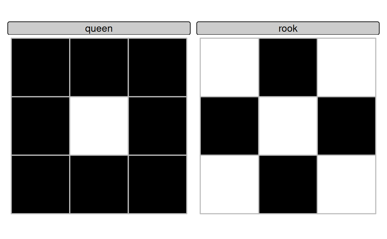
library(spdep)

#this creat the "graph", not yet the matrix
nb_q <- poly2nb(
  boston_utm,
  queen = TRUE
)

class(nb_q)

[1] "nb"

nb_q[[1]]

[1]   2   3   6   8 311 313 314 369

nb_q[[2]]

[1] 1 3 4 6

card(nb_q) #how many neighbors per each polygon

Distance-based neighbors

Neighbor relations can also be defined using geographic distance.

Two observations are considered neighbors if:

\[ d_{min} < d_{ij} < d_{max} \]

where \(d_{min}\) and \(d_{max}\) are chosen by the researcher.

• Unlike contiguity, distance-based neighbors can be applied to both point-referenced and areal data.

• When working with areal data, distances are often computed between centroids.

• The choice of the distance band is conceptually similar to the cutoff used in Conley standard errors.

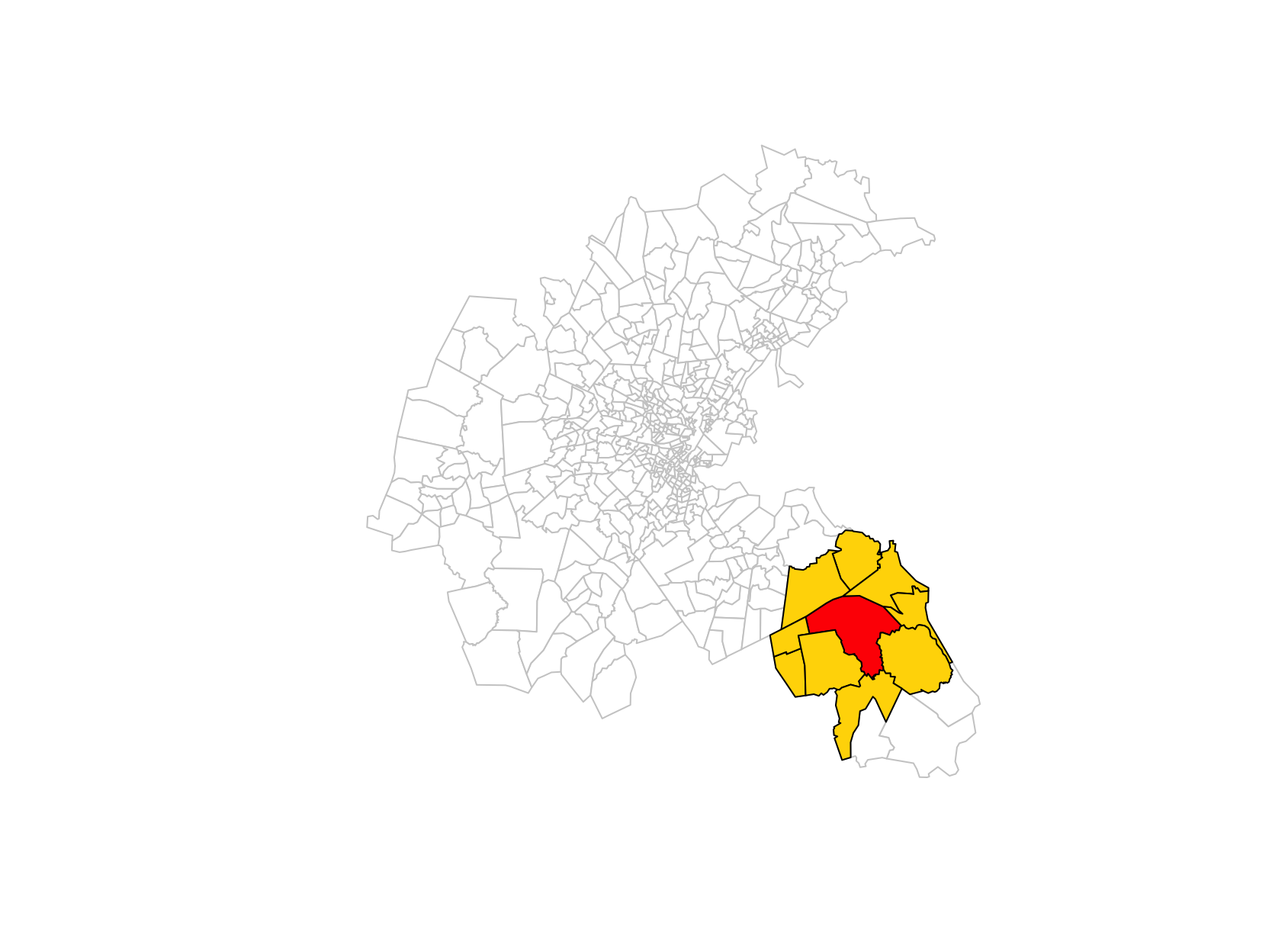
• Distance-based operations in spdep are generally safer in projected CRS.

nb_d <- dnearneigh(
  boston_utm_pts,
  0, #d_min
  10000 #d_max
)
nb_d[[499]]

[1] 492 495 496 497 498 500 501 502 505

nb_d[[500]]

[1] 492 495 499 501 502

k-nearest neighbors

• Distance bands may leave some observations without neighbors.

• A common alternative is k-nearest neighbors (kNN), where each observation is connected to its \(k\) closest neighbors.

• This ensures that every unit has at least \(k\) neighbors:

\[ N_i = \{j_1, j_2, \ldots, j_k\} \]

where \(N_i\) denotes the set of the \(k\) nearest neighbors of observation \(i\).

• Unlike distance bands, the resulting graph (and matrix) may be asymmetric: observation \(i\) may be among the nearest neighbors of \(j\), but not vice versa.

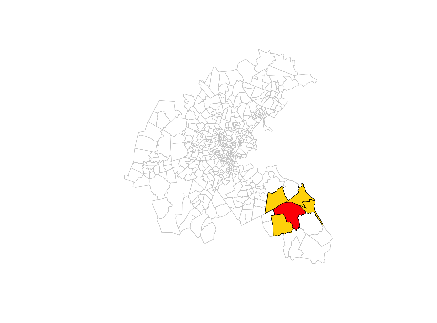
knn <- knearneigh(
  boston_utm_pts,
  k = 4
)

nb_knn <- knn2nb(knn)

nb_knn[[499]]

[1] 495 498 500 501

nb_knn[[495]]

[1] 486 488 489 494

From neighbor graphs to spatial weights matrices

A spatial weights matrix encode the binary information in the graph, plus the strength of spatial interactions.

              Polygons / points
                      ↓
        poly2nb(), dnearneigh(), knn2nb()
                      ↓
              Neighbor graph (nb)
                      ↓
                  nb2listw()
                      ↓
           Spatial weights matrix W

Different weighting schemes = different assumptions:

# Binary weights
lw_B <- nb2listw( #sparse representation of matrix (list)
  nb_q,
  style = "B"
)
lw_B$weights[[1]]

[1] 1 1 1 1 1 1 1 1

nb2mat(nb_q, style = "B")[1:5,1:5] #matrix representation

# Row-standardized weights
lw_W <- nb2listw(
  nb_q,
  style = "W"
)
lw_W$weights[[1]]

[1] 0.125 0.125 0.125 0.125 0.125 0.125 0.125 0.125

# Inverse-distance weights
d <- nbdists( #compute actual distances between neighbors (based on distance)
  nb_d,
  boston_utm_pts
)

nb_d[[499]]

[1] 492 495 496 497 498 500 501 502 505

d[[499]]

[1] 8361.259 6981.702 9082.101 8009.954 5338.481 6660.773 7131.115 7867.346
[9] 9236.959

idw <- lapply( #compute inverse distance
  d,
  function(x) 1/x
)

lw_id <- nb2listw( #create the sparse matrix with explicit weights
  nb_d,
  glist = idw,
  style = "B"
)

lw_id$weights[[499]]

[1] 0.0001195992 0.0001432316 0.0001101067 0.0001248447 0.0001873192
[6] 0.0001501327 0.0001402305 0.0001271077 0.0001082607

1/d[[499]]

[1] 0.0001195992 0.0001432316 0.0001101067 0.0001248447 0.0001873192
[6] 0.0001501327 0.0001402305 0.0001271077 0.0001082607

Spatial lags as operators

Once a spatial weights matrix \(\mathbf{W}\) has been defined, it can be used as an operator acting on variables.

• For any variable \(\mathbf{x}\), \(\mathbf{Wx}\) computes a (weighted) average of neighboring values.

• If \(\mathbf{W}\) is row-standardized, \((Wx)_i = \sum_j w_{ij}x_j\) can be interpreted as the (weighted) average value of variable \(x\) among the neighbors of unit \(i\).

• Examples:

  • \(\mathbf{Wy}\): neighboring outcomes;
  • \(\mathbf{WX}\): neighboring covariates;
  • \(\mathbf{W^2y}\): neighbors of neighbors.

• Spatial econometric models differ mainly in which spatial lag enters the model.

Suppose unit \(i\) has three neighbors:

y = [10, 20, 30]
weights = [0.2, 0.3, 0.5]

Its spatial lag is:

\[ Wy_i = 0.2 \times 10 + 0.3 \times 20 + 0.5 \times 30 = 23 \]

The spatial lag is therefore a weighted average of neighboring values.

lag_y <- lag.listw(
  lw_W,
  boston_utm$MEDV
)

head(lag_y)

[1] 28.70000 20.75000 28.76250 22.32500 34.82222 20.78333

Global Moran’s I

Global Moran’s I measures whether similar values tend to occur near each other in space.

Intuition:

High values near High values  → positive autocorrelation
Low values near Low values    → positive autocorrelation
High values near Low values   → negative autocorrelation

Moran’s I can be interpreted as the spatial analogue of a correlation coefficient. It combines:

• the values of the variable of interest;
• the spatial weights matrix \(\mathbf{W}\).

Values of Moran’s I are interpreted as:

\[ I > 0 \quad \text{positive spatial autocorrelation (clustering)} \]

\[ I \approx 0 \quad \text{absence of spatial autocorrelation} \]

\[ I < 0 \quad \text{negative spatial autocorrelation (dispersion)} \]

Once a spatial weights matrix (\(W\)) has been specified, Moran’s I provides a formal test of spatial autocorrelation.

moran.test(
  boston_utm$MEDV,
  lw_W
)
moran.test(
  resid(m),
  lw_W
)

\[ H_0:\ \text{no spatial autocorrelation} \qquad (I \approx E[I]=-1/(n-1)) \]

Variable	Moran’s I	p-value
MEDV	0.63	< 0.001
OLS residuals	0.49	< 0.001

In particular, Moran’s I measures the association between a variable and its spatial lag.

Moran scatterplot

The Moran scatterplot relates the value observed in a location to the average value observed among its neighbors.

• X axis: standardized variable \(z_i\);
• Y axis: its spatial lag \((Wz)_i\).

Formally, Moran’s I is given by

\[ I=\frac{n}{S_0} \frac{\mathbf z'W\mathbf z} {\mathbf z'\mathbf z} \]

where: \(S_0=\sum_i\sum_j w_{ij}\) is the sum of all spatial weights (\(n\) if \(W\) is row-standardized)

• The term \(\mathbf z'W\mathbf z\) measures whether nearby observations tend to have similar values.
• With row-standardized weights, Moran’s I coincide with the slope of the regression \(Wz \sim z\).

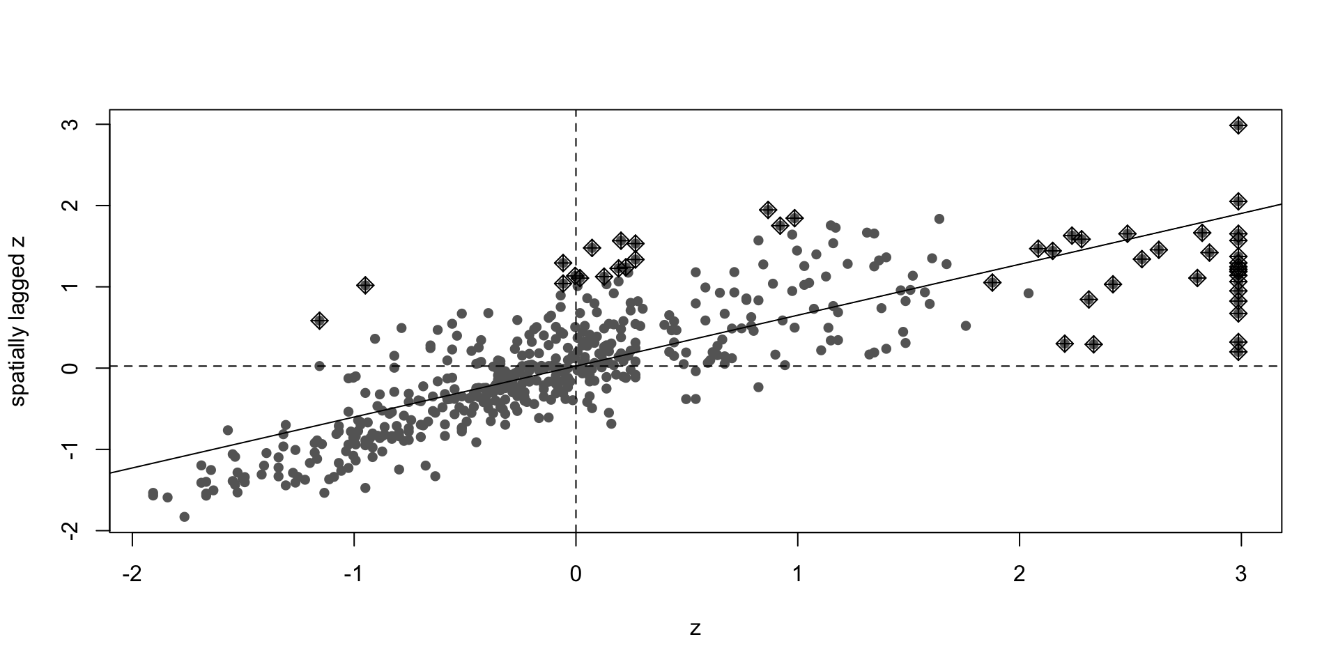
z <- scale(boston_utm$MEDV)[,1]
moran.plot(
  z,
  lw_W,
  labels = FALSE,
  pch = 16,
  col = "grey40"
)

• High–High (HH): clusters of high values;
• Low–Low (LL): clusters of low values;
• High–Low (HL): spatial outliers;
• Low–High (LH): spatial outliers.

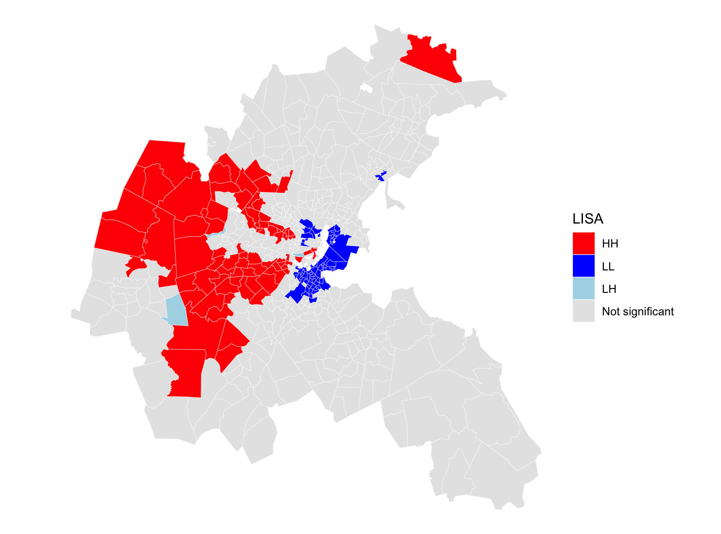
Local Indicators of Spatial Association (LISA)

Global Moran’s I summarizes spatial autocorrelation using a single number.

However, spatial dependence is often heterogeneous across space.

LISA decomposes global Moran’s I into observation-specific contributions:

\[ I_i = z_i (Wz)_i \]

where:

• \(z_i\) is the standardized value in location \(i\);
• \((Wz)_i\) is its spatial lag.

LISA therefore identifies where spatial clustering occurs.

lisa <- localmoran(boston_utm$MEDV,lw_W)
head(lisa,2)

           Ii          E.Ii      Var.Ii       Z.Ii Pr(z != E(Ii))
1 -0.34575085 -5.254157e-04 0.032753760 -1.9075336     0.05645152
2  0.01758754 -1.626873e-05 0.002045711  0.3892105     0.69712044

A LISA map can be thought of as the Moran scatterplot projected back into geographic space.

Choosing a spatial model

Spatial diagnostics can reveal spatial dependence, but they rarely identify its source. A possible empirical workflow is:

Estimate OLS
      ↓
Diagnose spatial dependence
      ↓
Formulate a theoretical mechanism
      ↓
Estimate and compare spatial models

Mechanism	Model	Equation
Shared shocks / correlated errors	SEM	\(y=X\beta+u\) \(u=\lambda Wu+\varepsilon\)
Neighboring covariates matter	SLX	\(y=X\beta+WX\theta+\varepsilon\)
Neighboring outcomes matter	SAR	\(y=\rho Wy+X\beta+\varepsilon\)

Diagnostics can provide useful guidance:

Question	Test in R
Residual spatial dependence?	moran.test(resid(m), lw_W), localmoran()
SAR or SEM?	lm.RStests(m, lw_W)

There is no general diagnostic test for SLX.

In practice, SLX is often used as a flexible starting point because it imposes weaker assumptions (and is less sensitive to \(\mathbf{W}\)):

• SAR assumes that outcomes directly affect neighboring outcomes, creating feedback loops and simultaneity;
• SEM assumes that unobserved shocks follow a spatial process;
• SLX only assumes that neighboring covariates affect local outcomes.

SLX: Spatial Lag of X

The SLX model assumes that neighboring characteristics directly affect local outcomes.

Examples:

• Air pollution in nearby municipalities affects local health;
• A storm in Pisa affects agricultural income in Livorno;
• Nearby amenities affect housing prices.

The model augments OLS with spatially lagged covariates:

\[ \mathbf y= \mathbf X\beta+ \mathbf{WX}\theta+ \varepsilon \]

where:

• \(\mathbf X\) contains local covariates;
• \(\mathbf{WX}\) contains neighboring covariates.

SLX therefore models spatial spillovers in explanatory variables.

Interpretation: \(\beta\): direct effects; \(\theta\): spillover effects.

boston_utm$W_CRIM <-
  lag.listw(
    lw_W,
    boston_utm$CRIM
  )

boston_utm$W_LSTAT <-
  lag.listw(
    lw_W,
    boston_utm$LSTAT
  )

slx <- lm(
  MEDV ~
    CRIM + RM + NOX + LSTAT +
    W_CRIM + W_LSTAT,
  data = boston_utm
)

moran.test(resid(slx),lw_W)

#We need lat lon to use conley, reproject
boston_wgs <- st_transform(boston_utm, 4326)
coords <- st_coordinates(
  st_centroid(boston_wgs)
)
boston_wgs$lon <- coords[,1]
boston_wgs$lat <- coords[,2]


slx <- feols(
  MEDV ~ CRIM + RM + NOX + LSTAT +
    W_CRIM + W_LSTAT,
  data = boston_wgs
)

summary(
  slx,
  vcov = vcov_conley(
    lat = "lat",
    lon = "lon",
    cutoff = 2
  )
)

Variable	OLS	SLX	SLX + Conley
CRIM	-0.103**	-0.089*	-0.089*
RM	5.219***	5.253***	5.253**
NOX	-0.122	3.161	3.161
LSTAT	-0.577***	-0.426***	-0.426**
W_CRIM	—	0.062	0.062
W_LSTAT	—	-0.319***	-0.319*
Adj. \(R^2\)	0.643	0.651	0.651

SAR: Spatial Autoregressive Model

The SAR model assumes that outcomes directly interact across space.

Examples:

• housing prices in nearby neighborhoods;
• crime diffusion;
• epidemics and contagion processes.

The model is:

\[ \mathbf y= \rho \mathbf{Wy} +\mathbf X\beta +\varepsilon \]

• \(\mathbf{Wy}\) is the spatial lag of the outcome;
• \(\rho\) measures the strength of spatial dependence.

Unlike SLX, SAR generates feedback loops: shocks propagate through the spatial network

       B         A affects B
      ↗ ↘        B affects C
     ↗   ↘       C affects A
    A ← ← C   

The model cannot be estimated by OLS because \(\mathbf{Wy}\) is endogenous. Maximum likelihood jointly estimates \(\rho\) and \(\beta\).

library(spatialreg)

sar <- lagsarlm(
  MEDV ~ CRIM + RM +
    NOX + LSTAT,
  data = boston_utm,
  listw = lw_W
)

Coefficients:
              Estimate   p-value
CRIM           -0.046     0.085
RM              4.514    <0.001 ***    SAR coefficients are NOT marginal effects
NOX             3.543     0.101
LSTAT          -0.304    <0.001 ***

Rho: 0.54666, LR test value: 188.84, p-value: < 2.22e-16 #strong positive spatial dependence feedbacks
AIC: 2980.4, (AIC for lm: 3167.2) #model fit has improved
LM test for residual autocorrelation
test value: 37.175, p-value: 1.0799e-09 #still spatial dependence remaining

To retrieve marginal effects:

imp <- impacts(
  sar,
  listw = lw_W,
  R = 1000
)
summary(imp, zstats = TRUE)

Impact measures (lag, exact):
                 Direct    Indirect      Total
CRIM dy/dx  -0.04931722 -0.05197838 -0.1012956
RM dy/dx     4.84834130  5.10995709  9.9582984
NOX dy/dx    3.80478493  4.01009058  7.8148755
LSTAT dy/dx -0.32697440 -0.34461789 -0.6715923

Direct   : what happens locally?
Indirect : what happens on average elsewhere?
Total    : what happens overall?

SEM: Spatial Error Model

The SEM model assumes that spatial dependence arises from unobserved factors.

Examples:

• school quality;
• environmental conditions;
• historical development;
• local institutions.

The model is:

\[ \mathbf y=\mathbf X\beta+\mathbf u \qquad \text{with} \qquad \mathbf u= \lambda \mathbf{Wu} +\varepsilon \] where \(\lambda\) measures spatial dependence in unobserved shocks.

Unlike SAR, outcomes do not directly interact.

Shared unobserved factors → Spatially correlated errors → Housing prices

SEM is conceptually close to Conley:

• Conley: robust inference;
• SEM: explicit modeling of spatial errors.

sem <- errorsarlm(
  MEDV ~ CRIM + RM +
    NOX + LSTAT,
  data = boston_utm,
  listw = lw_W
)

Coefficients:
              Estimate   p-value
CRIM          -0.098    <0.001 ***
RM             5.351    <0.001 ***
NOX          -17.317    <0.001 ***
LSTAT         -0.393    <0.001 ***

λ = 0.765***     strong spatial dependence
                 in unobserved factors

AIC: 2914        (OLS: 3167)
                 (SAR: 2980)
                 better model fit

Interpretation:

• Nearby tracts appear to share omitted factors affecting housing prices.
• The estimated effect of NOX becomes much larger after accounting for spatially correlated omitted factors \(\rightarrow\) spatial OVB.
• Unlike SAR, SEM does not generate feedback loops \(\rightarrow\) coefficients retain their usual marginal interpretation.

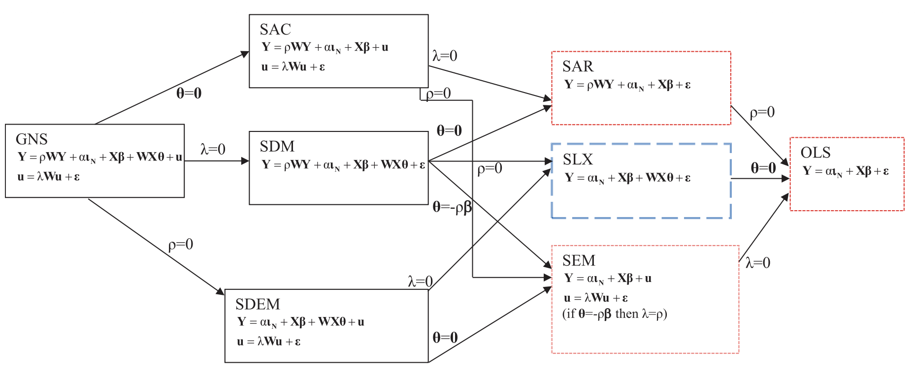
A large family of models

Comparison of Different Spatial Econometric Model Specifications (Source: Vega and Elhorst 2015)

Beyond cross-sections: panel data and DiD

Panel data

Fixed effects already absorb many sources of spatial dependence:

\[ y_{it}=X_{it}\beta+\mu_i+\tau_t+\varepsilon_{it} \]

\(\mu_i\) absorbs time-invariant local characteristics (e.g. geography, institutions). Spatial spillovers may still remain (e.g. pollution in one area may affect nearby areas.)

• SLX model naturally extends to panel settings:

m <- feols(
  y ~ X + WX |
    unit + year,
  data,
    vcov = vcov_conley(
    lat = "lat",
    lon = "lon",
    cutoff = 100
  )
)

• acreg (Stata): robust inference under spatial and serial correlation.
• splm (R): panel estimators for SAR and SEM models.

Difference-in-Differences

Standard DiD assumes that untreated units are not affected by treatment.

Spatial spillovers may violate this assumption:

Treatment in A → Outcome in B

Example:

New subway station in A
        ↓
Housing prices increase also in B

In this case, B is no longer a pure control unit.

Possible approaches include:

• use Conley standard errors for spatially correlated errors;
• include spatial lags of treatment (SLX);
• define treatment exposure using distance-based measures;
• estimate dedicated spatial DiD models.

Suggested references

Textbooks

• Bivand, R. S., Pebesma, E. & Gómez-Rubio, V. (2013). Applied Spatial Data Analysis with R (2nd ed.). Springer.
• LeSage, J. P. & Pace, R. K. (2009). Introduction to Spatial Econometrics. Chapman & Hall/CRC.
• Anselin, L. & Rey, S. J. (2014). Modern Spatial Econometrics in Practice: A Guide to GeoDa, GeoDaSpace and PySAL. GeoDa Press.
• Elhorst, J. P. (2014). Spatial Econometrics: From Cross-Sectional Data to Spatial Panels. Springer.
• Anselin, L. (1988). Spatial Econometrics: Methods and Models. Kluwer Academic.

Key papers

• Conley, T. G. (1999). “GMM Estimation with Cross Sectional Dependence.” Journal of Econometrics, 92(1), 1–45.
• Vega, S. H. & Elhorst, J. P. (2015). “The SLX Model.” Journal of Regional Science, 55(3), 339–363.
• Colella, F., Lalive, R., Sakalli, S. O. & Thoenig, M. (2023). acreg: Arbitrary correlation regression. Stata Journal, 23(1), 119–147.