Spatial Data Analysis

Applied spatial workflows

Sant’Anna School of Advanced Studies

Matteo Coronese
m.coronese@santannapisa.it

June 2026

What will we learn in this course?

Lecture 1 - Spatial data basics

Lecture 2 — Operating with spatial datasets

Lecture 3 — Elements of spatial dependence and econometrics

Lecture 4 — Applied spatial workflows

• Exposure variables
• Temporal and spatial harmonization
• Raster-vector interactions
• Panel construction
• Climate econometrics

First things first: get the data!

Go to https://l1nk.dev/tvfd8zx

From global rasters to econometric panels

Working with spatial data often requires much more than simply fitting a regression model.

Researchers routinely need to:

• combine multiple spatial datasets;
• harmonize different grids and resolutions;
• aggregate information over administrative units;
• define meaningful weighting schemes;
• construct variables suitable for statistical analysis.

The exact workflow depends on the research question, but these operations appear repeatedly across many disciplines.

One of the most common tasks is the construction of an exposure variable.

What is an exposure variable?

An exposure variable quantifies how much an observational unit is exposed to a spatial phenomenon.

Examples:

Unit	Spatial phenomenon	Exposure variable
Country	Temperature	Population-weighted temperature
Municipality	PM2.5	Population exposure to pollution
Household	Flood hazard	Flood risk
Region	Transport infrastructure	Market accessibility

Exposure variables are rarely directly observed.

Instead, they are constructed by combining spatial information with aggregation rules and weighting schemes.

• Case study: Burke, Hsiang & Miguel (Nature, 2015)

• A highly influential paper in climate economics that uses spatial data to estimate the effect of temperature on economic growth.

A general workflow

• Climate is only one application: the same workflow can be used to study pollution, accessibility, flood risk, or habitat loss.

• The analytical choices made during construction can strongly influence scientific conclusions.

• Goal of today’s lecture: transform raw spatial data into scientific inference.

ERA5 climate data

We start from ERA5 reanalysis data, the gold standard in modern climate analysis.

We focus on data on temperature and precipitation.

• Load temp.tif and prec.tif. Function rast()

• Inspect the raster: crs(), res(), extent(), names().

What CRS are we using? What is the spatial resolution? What is the temporal resolution, since data is covering 1980-2025?

Names are cryptic…

• Use:

names(temp) <- as.POSIXct(
  as.numeric(sub(".*=", "", names(temp))),
  origin = "1970-01-01",
  tz = "UTC"
)

to have nicer names.

• Do the same for prec.

Climate units matter

• Inspect the first monthly layer: use global() with min and max

global(temp[[1]], c("min", "max"), na.rm = TRUE)

What’s the unit for temperature?

temp <- temp - 273.15

• do the same for prec.

global(prec[[1]], c("min", "max"), na.rm = TRUE)

Does the maximum look reasonable?

Aggregate temperature over time

To aggregate over time, you can use the function tapp

tapp(
  rast, #the raster object
  years, #a grouping vector, the same length as nlyr(rast)
  mean #aggregating function
)

You can retrieve the years vector using the lubridate function

years <- format(
  as.Date(names(temp)),
  "%Y"
)

Should annual temperature be computed trough a mean or a sum?

temp_year <- tapp(
  temp, #compute month totals
  years, #over years
  mean #average across months
)

Aggregate precipitation over time

Temperature and precipitation behave differently.

Variable	Type	Annual aggregation
Temperature	Intensive	?
Precipitation	Extensive	?

Should we use sum() or mean()? Should we multiply our values by something before aggregating?

days <- days_in_month(
  as.Date(names(prec))
)

prec_year <- tapp(
  prec * days, #compute month totals
  years, #over years
  sum #sum over months
) * 1000 #transform into mm

Sanity checks

• Inspect the new rasters temp_year and temp_year by computing min, mean and max through global():
  • Temperature: roughly between -50°C and +40°C
  • Precipitation: it is measured in mm now…
• Plot random years: Can you recognize: deserts, mountain ranges, tropical regions?

global(temp_year, c("min", "mean", "max"))
global(prec_year, c("min", "mean", "max"))

plot(temp_year[[1]])
title("ERA5 Temperature, 1980")

plot(prec_year[[1]])
title("ERA5 Precipitation, 1980")

Better be safe than sorry… Never trust transformations without checking the output.

Population data

“If a tree falls in a forest and no one is around to hear it, does it make a sound?”

• People tend to concentrate in cities, valleys, and coastal areas. For economic analysis, we only care about climate experienced by people (e.g. we don’t care how hot is in a desert).

• To account for this, we also need information on where people live.

• Data source is Gridded Population of the World (GPW v4, NASA), for 2000, 2005, 2010, 2015, 2020.

• Load each of the five rasters using rast.

• Combine them in a single raster using rast(list(...)).

• Fix layer names.

pop2000 <- rast(
  "data/gpw_v4_population_count_adjusted_to_2015_unwpp_country_totals_rev11_2000_2pt5_min.tif"
)

pop2005 <- rast(
  "data/gpw_v4_population_count_adjusted_to_2015_unwpp_country_totals_rev11_2005_2pt5_min.tif"
)

#...

pop <- rast(
  list(
    pop2000, pop2005, pop2010, pop2015, pop2020
  )
)

names(pop) <- c("2000", "2005", "2010", "2015", "2020")

Sanity check: Does the population raster make sense?

Inspect the raster:

• plot()
• global()

Question:

Can we recover world population totals?

Expected values:

• 2000 ≈ 6.1 billion
• 2005 ≈ 6.5 billion
• 2010 ≈ 6.9 billion
• 2015 ≈ 7.3 billion
• 2020 ≈ 7.8 billion

global(pop, "sum", na.rm = TRUE) / 1e9

Temporal harmonization

We need climate and population rasters to talk to each other.

• The GPW dataset provides population counts for 2000, 2005, 2010, 2015, 2020.

• Climate data are annual: 1980 … 2025.

We assume that population changes linearly over time.

Our strategy:

• 1980–1999 → use 2000 population
• 2000–2020 → linear interpolation
• 2021–2025 → use 2020 population

Construct a raster for population in 2003 manually.

2000 -- -- -- 2003 -- -- 2005
 |              |          |
 0%            60%       100%

pop2003 <-
  0.4 * pop[["2000"]] +
  0.6 * pop[["2005"]]

–

Build a general interpolation function

Let’s automate, building a custom function

interp_rast <- function(year, rast){
  
  if(year <= 2000) # before 2000: use 2000 population
    return(rast[["2000"]])
  
  if(year >= 2020) # after 2020: use 2020 population
    return(rast[["2020"]])
  
  y0 <- floor(year / 5) * 5 # lower and upper benchmark years
  y1 <- y0 + 5
  
  weight_next <- # interpolation weight
    (year - y0) /
    (y1 - y0)
  
  (1 - weight_next) * # linear interpolation
    rast[[as.character(y0)]] +
    
    weight_next *
    rast[[as.character(y1)]]
}

Test the function applying it to 2003 and use identical() to check if it is equal to pop2003

test <- interp_rast(2003, pop)
identical(test, pop2003)

Compute all years

• Build a vector years with the input variable (1980:2025)

years <- 1980:2025

• Use lapply to apply the function to every year

pop_yearly <- lapply(
  years,
  interp_rast,
  rast = pop
)

• Inspect the object with class() and length()

class(pop_yearly)
length(pop_yearly)
class(pop_yearly[[1]])

Why is the result a LIST? Because each element is a raster.

• Stack everything into a single raster object

pop_yearly <- rast(pop_yearly)

• Fix the names of the layers

names(pop_yearly) <- years

• Reinspect the object. How many layers do you expect?

class(pop_yearly)

nlyr(pop_yearly)

pop_yearly

• Perform a sanity check: compute global population by year

global(pop_yearly, "sum", na.rm = TRUE) / 1e9

Under which circumstances using 2000 population for 1980–1999 is potentially problematic?

Spatial harmonization

Climate and socio-economic data rarely share the same grid.

Before combining rasters, we must answer two questions:

1. Do they have the same resolution?
2. Are their cells aligned in space?

• Let’s start with resolution. Compare climate and population rasters using res(). What differences do you observe?

res(prec_year)
res(pop_yearly)

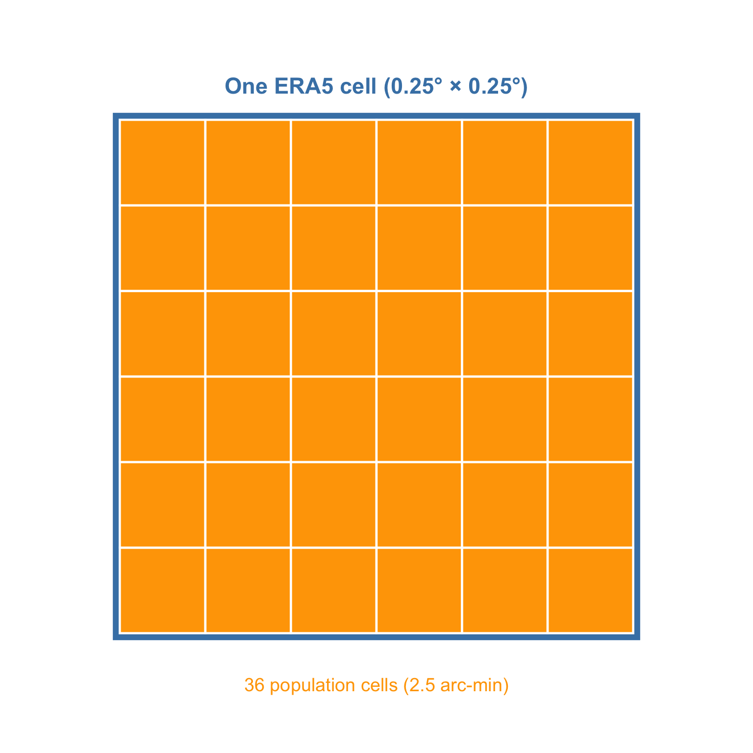
• Compute the ratio: how many cells from pop_yearly fit into a cell from prec_year?

res(prec_year)/res(pop_yearly)

Aggregating smaller raster

The empirical bottleneck is always given by the coarser dataset.

• Population is an extensive variable. When aggregating cells should we use sum() or mean()?

• Use the function aggregate to aggregate by a factor of six. Sintax:

aggregate(
  raster, #raster object
  fact = n, #factor of aggregation
  fun = "fun", #aggregating function
  na.rm = TRUE #options
)

pop_15 <- aggregate(
  pop_yearly,
  fact = 6,
  fun = "sum",
  na.rm = TRUE
)

• Sanity checks. Check the resolution of pop_15. Compare annual global population between pop_15 and pop_yearly.

res(pop_15)
global(pop_15, "sum", na.rm = TRUE) / 1e9
global(pop_yearly, "sum", na.rm = TRUE) / 1e9

Spatial harmonization: alignin grids

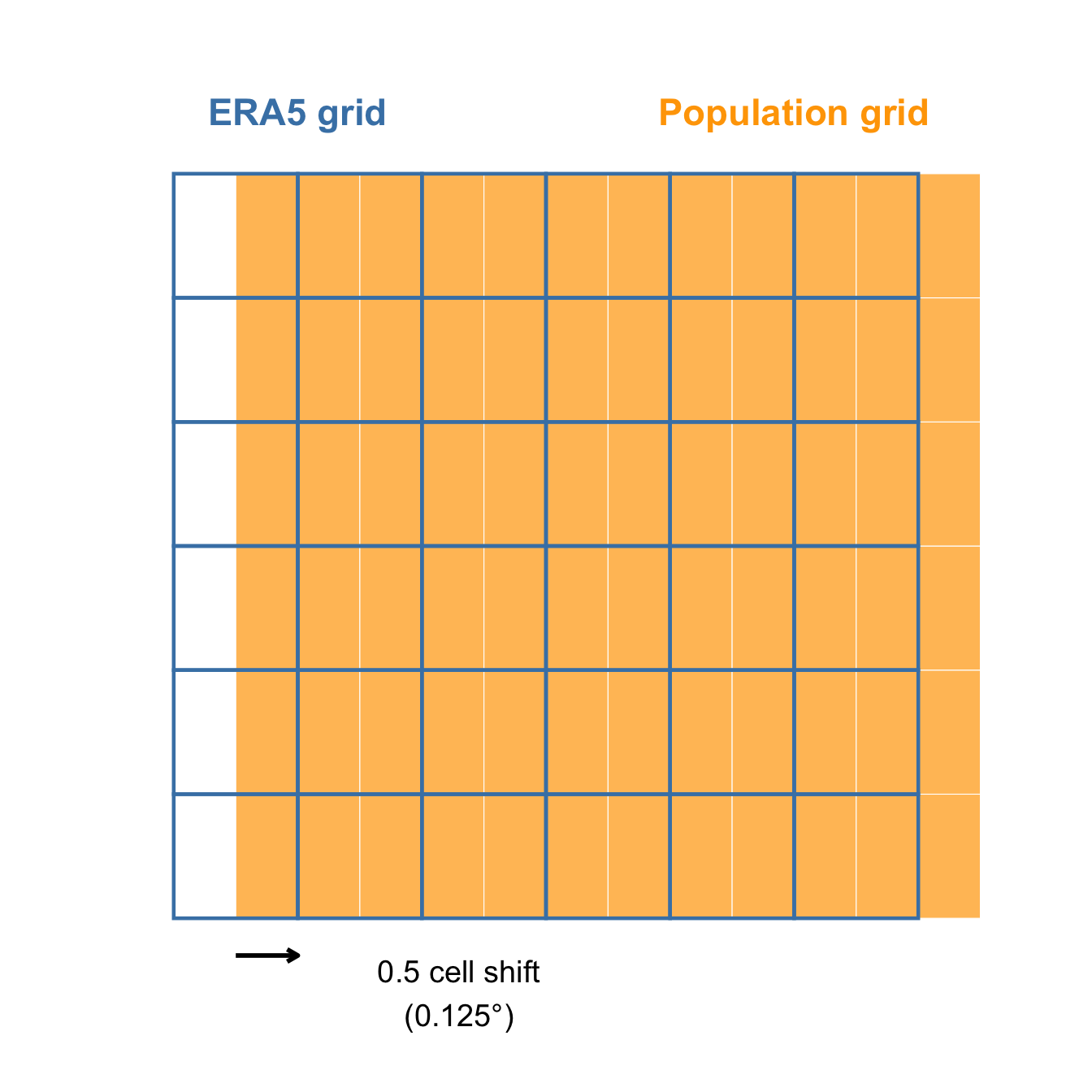
Our rasters now share the same resolution. But are they aligned?

• Check using ext() and origin().

ext(pop_15)
ext(prec_year)
origin(pop_15)
origin(prec_year)

The two rasters are misaligned both vertically and horizontally by half cell.

Spatial interpolation

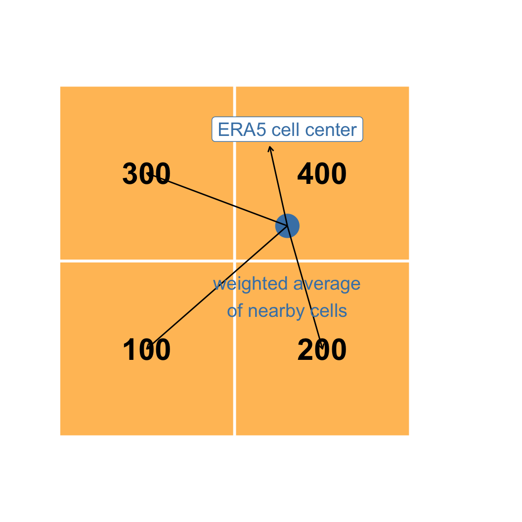
• A common fix to this problem is to interpolate values on one grid relative to the position of each cell in another grid.

• Among many methods, we are going to use the bilinear interpolation. We assign to each cell the average of the four nearest cells,

Use the command resample. Sintax:

resample(
  resampled_raster,
  target_raster,
  method = "bilinear"
)

pop_era5 <- resample(
  pop_15,
  prec_year,
  method = "bilinear"
)

• Sanity checks
  • Geometries should now match. Check with compareGeom.
  • World population totals should remain approximately unchanged.

compareGeom( pop_era5, prec_year, stopOnError = FALSE)
global(pop_era5, "sum", na.rm = TRUE) / 1e9

From rasters to countries

Until now we worked with rasters.

However, econometric analysis is often performed at the country level.

We therefore need country polygons to aggregate raster information.

First, download country polygons:

countries <- rnaturalearth::ne_countries(
  scale = "medium",
  returnclass = "sf"
)

• Use st_crs and crs to check compatibility
• Use plot() and plot(., add=TRUE) to have visual overlay confirmation

st_crs(countries)
crs(temp_year)
plot(prec_year[[1]])
plot(st_geometry(countries), add = TRUE)

Zonal statistics and exact extraction

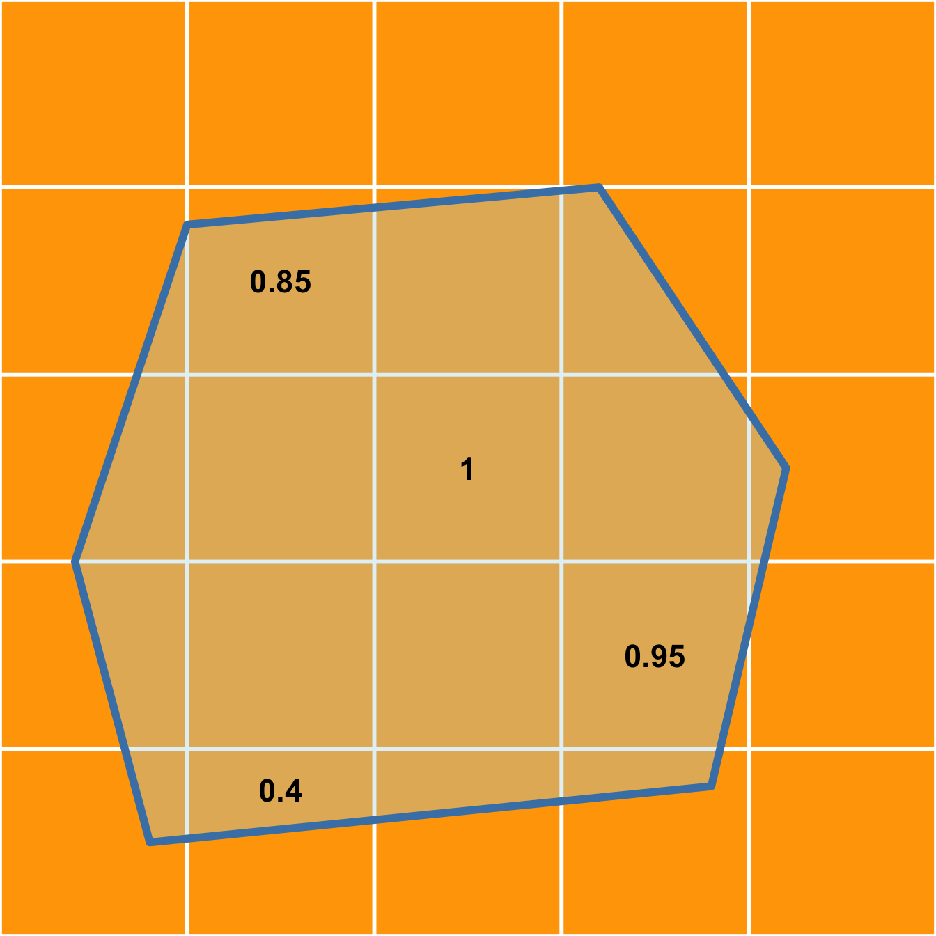
We now want to aggregate raster values over polygons. This operation is known as zonal statistics.

Cells intersecting country borders are only partially counted. Through exact extraction, boundary cells contribute proportionally to their covered area.

exact_extract(
  raster,
  polygon,
  fun #aggregating function
)

Further weighting: population weighting

We are not simply using zonal statistic, but a weighted (by population) version of it. A hot desert and a large city should not contribute equally.

Population-weighted temperature is defined as:

\[ T^{PW} = \frac{\sum_i T_i \times Pop_i} {\sum_i Pop_i} \]

where (i) indexes raster cells.

• First compute the denominator \(T_i \times Pop_i\) for every raster cell:

temp_pop <- temp_year * pop_era5
prec_pop <- prec_year * pop_era5

• Then, extract them and the denominator (pop_era5) using exact_exctract(). Which aggregating function should we use?

temp_num <- exact_extract(
  temp_pop,
  countries,
  "sum"
)

prec_num <- exact_extract(
  prec_pop,
  countries,
  "sum"
)

pop_den <- exact_extract(
  pop_era5,
  countries,
  "sum"
)

Further weighting: population weighting II

• At this point, simply build the weighted measures conmputing the ratios

temp_pw <- temp_num / pop_den
prec_pw <- prec_num / pop_den

• Sanity check: check dimensions with dim() and inspect values with summary()

dim(temp_pw)
dim(prec_pw)

summary(as.matrix(temp_pw))
summary(as.matrix(prec_pw))

• Do they make sense?

• Use the function colMeans(., na.rm = TRUE) to inspect and plot average temperature by year. We should see an increase…

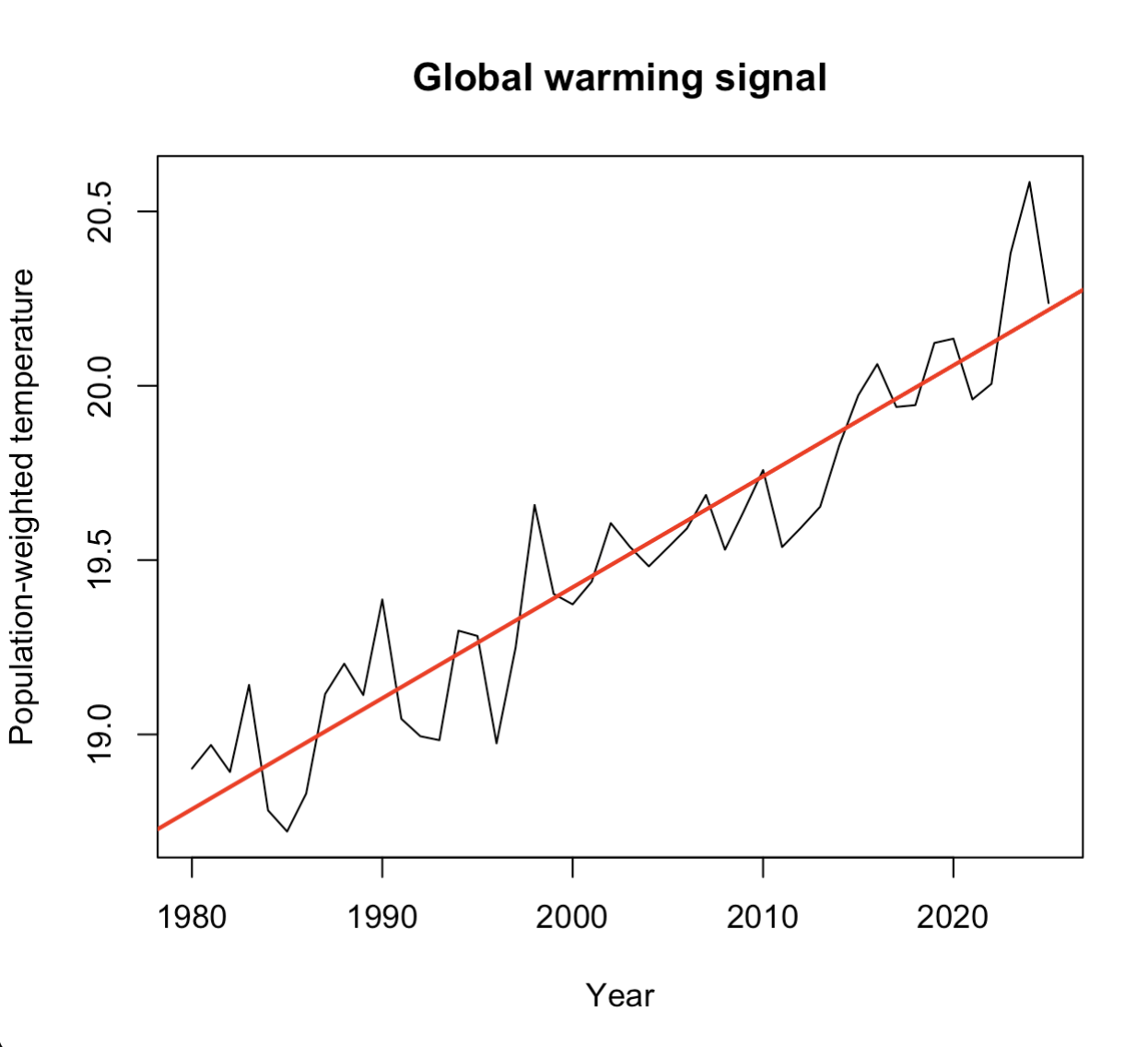
Is this evidence of climate change? Of course a bit, but not necessarily: population weights also evolve over time.

Housekeeping

• Remove NA’s

keep <- !apply(is.na(temp_pw), 1, all)

countries <- countries[keep, ]
temp_pw   <- temp_pw[keep, ]
prec_pw   <- prec_pw[keep, ]

temp_df <- as.data.frame(temp_pw)
prec_df <- as.data.frame(prec_pw)

years <- 1980:2025

names(temp_df) <- paste0("temp_", years)
names(prec_df) <- paste0("prec_", years)

• Use the command cbind to attach temp_df and prec_df columns to countries

countries %>%
  st_drop_geometry() %>%
  transmute(
    iso3 = adm0_a3, #we call the identifies iso3
    country = name  
  ) %>%
  bind_cols(
    temp_df,
    prec_df,
  )

• For most econometric software, you need data in long format. Inspect the names of you columns and use pivot_longer()

names(panel_wide)

panel <- panel_wide %>%
  pivot_longer(
    cols = -c(iso3, country),
    names_to = c(".value", "year"),
    names_sep = "_"
  ) %>%
  mutate(
    year = as.integer(year)
  )

Economic data

-vNow, we only need GDP data. Dowload it from the World Bank repository:

gdp <- WDI::WDI(
  country = "all",
  indicator = "NY.GDP.PCAP.PP.KD",
  start = 1980,
  end = 2025
)

• Perform a left_join() with you object panel

panel <- panel %>%
  left_join(
    gdp %>% select(iso3c, year, NY.GDP.PCAP.PP.KD),
    by = c("iso3" = "iso3c", "year")
  )

• Use filter() to remove observations without GDP information

panel <- panel %>%
  filter(
    !is.na(NY.GDP.PCAP.PP.KD)
  )

• Use group_by() and mutate() to compute the rate of growth of GDP:

panel <- panel %>%
  arrange(
    iso3,
    year
  ) %>%
  group_by(iso3) %>%
  mutate(
    growth = 100 * (
      log(NY.GDP.PCAP.PP.KD) -
        lag(log(NY.GDP.PCAP.PP.KD))
    )
  ) %>%
  ungroup()

• Sanity checks: are these growth rates reasonable? Use summary()

summary(panel$growth)
quantile(
  panel$growth,
  probs = c(.01, .05, .5, .95, .99),
  na.rm = TRUE
)

Why a quadratic specification?

Now we have built our panel with exposure variables. In Burke, Hsiang & Miguel (2015), the question is:

Does temperature affect economic growth?

They further argue that such relationship is non-linear.

• Very cold countries may benefit from warming.

• Very hot countries may be harmed.

A simple way to capture this idea is:

\[ \text{growth} = \beta_1 T + \beta_2 T^2 \]

• Why growth?
• Which sign would you expect for \(\beta_2\)?

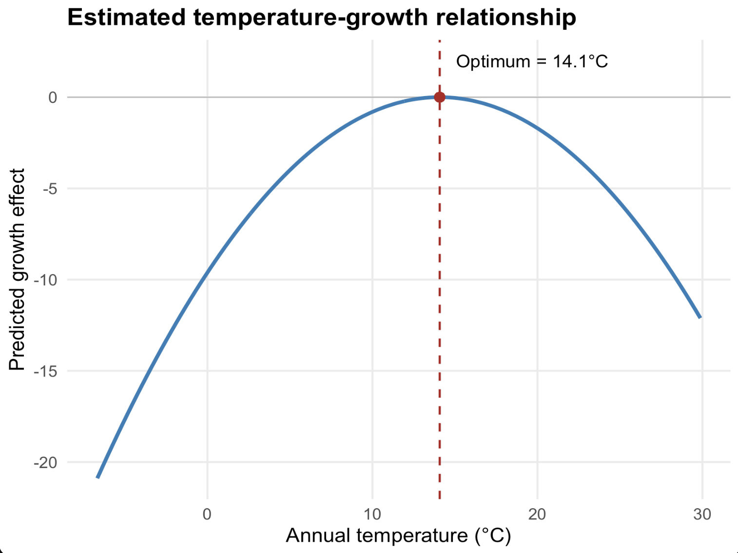
If \((\beta_2 < 0)\), the relationship is hump-shaped. Temperature can increase growth up to a point, and reduce it afterwards.

Empirical specification

\[ g_{it} = \beta_1 T_{it} + \beta_2 T_{it}^2 + \beta_3 P_{it} + \beta_4 P_{it}^2 + \alpha_i + \lambda_t + \delta_i t + \gamma_i t^2 + \varepsilon_{it} \]

where:

• \(g_{it}\): GDP per capita growth
• \(T_{it}\): temperature exposure
• \(P_{it}\): precipitation exposure

Why country fixed effects \((\alpha_i)\)?

To absorb time-invariant country characteristics:

• geography;
• institutions;
• culture;
• average climate.

Why year fixed effects \((\lambda_t)\)?

To absorb global shocks affecting all countries:

• oil crises;
• business cycles;
• technological change.

Why country-specific trends \((\delta_i t + \gamma_i t^2)\)?

To remove slow-moving country-specific processes.

• economic convergence;
• demographic transition;
• institutional reforms.

We allow each country to follow its own smooth trajectory.

Where does identification come from?

After all these controls, the model is identified from:

year-to-year climate fluctuations within a country

We are not comparing:

• Italy vs Norway
• Brazil vs Sweden

We are comparing:

• Italy in warmer years vs cooler years
• Brazil in warmer years vs cooler years

while controlling for long-run trends and global shocks.

Estimating the model

Use feols() to estimate the Burke specification.

General syntax:

feols(
  y ~ x1 + x2 + ... |
    fe_1 + fe_2,
  data = data,
  cluster = ~unit
)

For this exercise:

• dependent variable: growth
• climate variables: temp, temp^2, prec, prec^2
• country fixed effects: iso3
• year fixed effects: year
• cluster variable: iso3

To include country-specific polynomial trends, use:

iso3[t + I(t^2)]

which estimates, for each country, \(\alpha_i + \delta_i t + \gamma_i t^2\)

m1 <- feols(
  growth ~ temp + I(temp^2) +
    prec + I(prec^2) |
    iso3[t + I(t^2)] + year,
  data = panel,
  cluster = ~iso3
)

• Why include precipitation?
• Why include quadratic terms?
• Why cluster standard errors by country?
• Use coef() to retrieve estimated coefficients and compute the vertex of the parabola (\(v=-\beta1_/(2\beta_2)\)).
• Is the estimated optimum close to the original ~13°?

-coef(m1)["temp"]/(2*coef(m1)["I(I(temp^2))"])

Winsorizing - Extreme growth episodes

• Iraq 1991 (war); Equatorial Guinea 1997 (oil discovery).
• Other possible outliers from political collapses, measurement errors.

Why are outliers potentially problematic?

• OLS squares residuals. Large observations therefore receive disproportionate weight.
• Our specification also contains quadratic climate terms. Extreme observations may therefore have a strong influence on the estimated curve.

Solution: winsorize growth

panel2 <- panel %>%
  mutate(
    growth_w = pmax(
      pmin(growth, 15),
      -15
    )
  )

Re-estimate the model:

m2 <- feols(
  growth_w ~ temp + I(temp^2) +
    prec + I(prec^2) |
    iso3[ t + I(t^2) ] + year,
  data = panel2,
  cluster = ~iso3
)